8.4.3. Application to a stellar image

8.4.3.1. Data used in this notebook

The image in this notebook is of the field of the star TIC 125489084 on a night when the moon was nearly full. The moonlight caused a smooth gradient across the background of the image.

As discussed in the section about background subtraction with this image, the best way to remove the background in this case is to use photutils to construct a 2D model of the background.

As we will see shortly, image segmentation doesn’t significantly improve source detection in this case, since all of the sources are stars.

import warnings

from astropy.convolution import convolve
from astropy.nddata import CCDData
from astropy.stats import sigma_clipped_stats, SigmaClip
import astropy.units as u
from astropy.visualization import ImageNormalize, LogStretch, AsymmetricPercentileInterval

import matplotlib.pyplot as plt
from matplotlib.ticker import LogLocator

import numpy as np

from photutils.aperture import EllipticalAperture
from photutils.background import Background2D, MeanBackground
from photutils.centroids import centroid_2dg
from photutils.detection import find_peaks, DAOStarFinder, IRAFStarFinder
from photutils.segmentation import detect_sources, make_2dgaussian_kernel, SourceCatalog

# Show plots in the notebook
%matplotlib inline

In the next cell, we read the data, mask out the edges and subtract the two dimensional background.

ccd_image = CCDData.read('TIC_125489084.01-S001-R055-C001-ip.fit.bz2')

# Create a mask array
mask = np.zeros_like(ccd_image, dtype=bool)

# Set the mask for a border of 50 pixels around the image
mask[:50, :] = mask[-50:, :] = mask[:, :50] = mask[:, -50:] = 1.0

ccd_image.mask = mask

sigma_clip = SigmaClip(sigma=3., maxiters=5)
bkg_estimator = MeanBackground()
bkg = Background2D(ccd_image, box_size=200, filter_size=(9, 9), mask=ccd_image.mask,
                   sigma_clip=sigma_clip, bkg_estimator=bkg_estimator)
# Calculate the 2D background subtraction, maintaining metadata, unit, and mask
ccd_2d_bkgdsub = ccd_image.subtract(bkg.background)

data_subtracted = ccd_2d_bkgdsub.data

WARNING: FITSFixedWarning: RADECSYS= 'FK5 ' / Equatorial coordinate system 
the RADECSYS keyword is deprecated, use RADESYSa. [astropy.wcs.wcs]

mean, median, std = sigma_clipped_stats(data_subtracted.data, sigma=3.0, maxiters=5)

plt.style.use('../photutils_notebook_style.mplstyle')

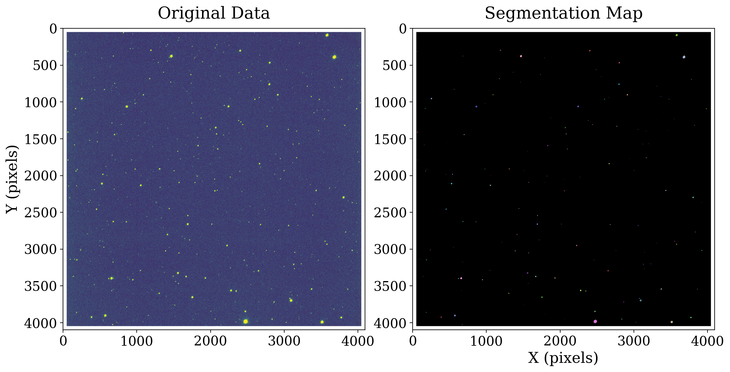
Next, we use image segmentation to find the sources.

# Define threshold and minimum object size
threshold = 5. * std
npixels = 10
fwhm = 5
kernel_size = 5
kernel = make_2dgaussian_kernel(fwhm, size=kernel_size)
convolved_data = convolve(data_subtracted.data, kernel, mask=ccd_2d_bkgdsub.mask)
# Create a segmentation image
segm = detect_sources(convolved_data, threshold, npixels, mask=ccd_2d_bkgdsub.mask)

print('Found {} sources'.format(segm.max_label))

Found 145 sources

WARNING: nan_treatment='interpolate', however, NaN values detected post convolution. A contiguous region of NaN values, larger than the kernel size, are present in the input array. Increase the kernel size to avoid this. [astropy.convolution.convolve]

This is roughly half the number of sources detected by star finding.

# Set up the figure with subplots
fig, [ax1, ax2] = plt.subplots(1, 2, figsize=(12, 6))
plt.tight_layout()

# Plot the data
# Set up the normalization and colormap
norm_image  = ImageNormalize(ccd_2d_bkgdsub, interval=AsymmetricPercentileInterval(30, 99.5))
cmap = plt.get_cmap('viridis')
cmap.set_bad('white') # Show masked data as white

# Plot the original data
fitsplot = ax1.imshow(np.ma.masked_where(ccd_2d_bkgdsub.mask, ccd_2d_bkgdsub),
                      norm=norm_image, cmap=cmap)
ax1.set_ylabel('Y (pixels)')
ax1.set_title('Original Data')

# Plot the segmentation image
segplot = ax2.imshow(np.ma.masked_where(ccd_image.mask, segm), vmin=1, cmap=segm.cmap)
ax2.set_xlabel('X (pixels)')
ax2.set_title('Segmentation Map')

# Define the colorbar
# cbar_ax = fig.add_axes([1, 0.09, 0.03, 0.87])
# cbar = plt.colorbar(segplot, cbar_ax)
# cbar.set_label('Object Label', rotation=270, labelpad=30)

Text(0.5, 1.0, 'Segmentation Map')

As in the previous notebook, we construct a SourceCatalog to obtain more information about the sources detected by segmentation.

catalog = SourceCatalog(ccd_2d_bkgdsub.data, segm)
table = catalog.to_table()

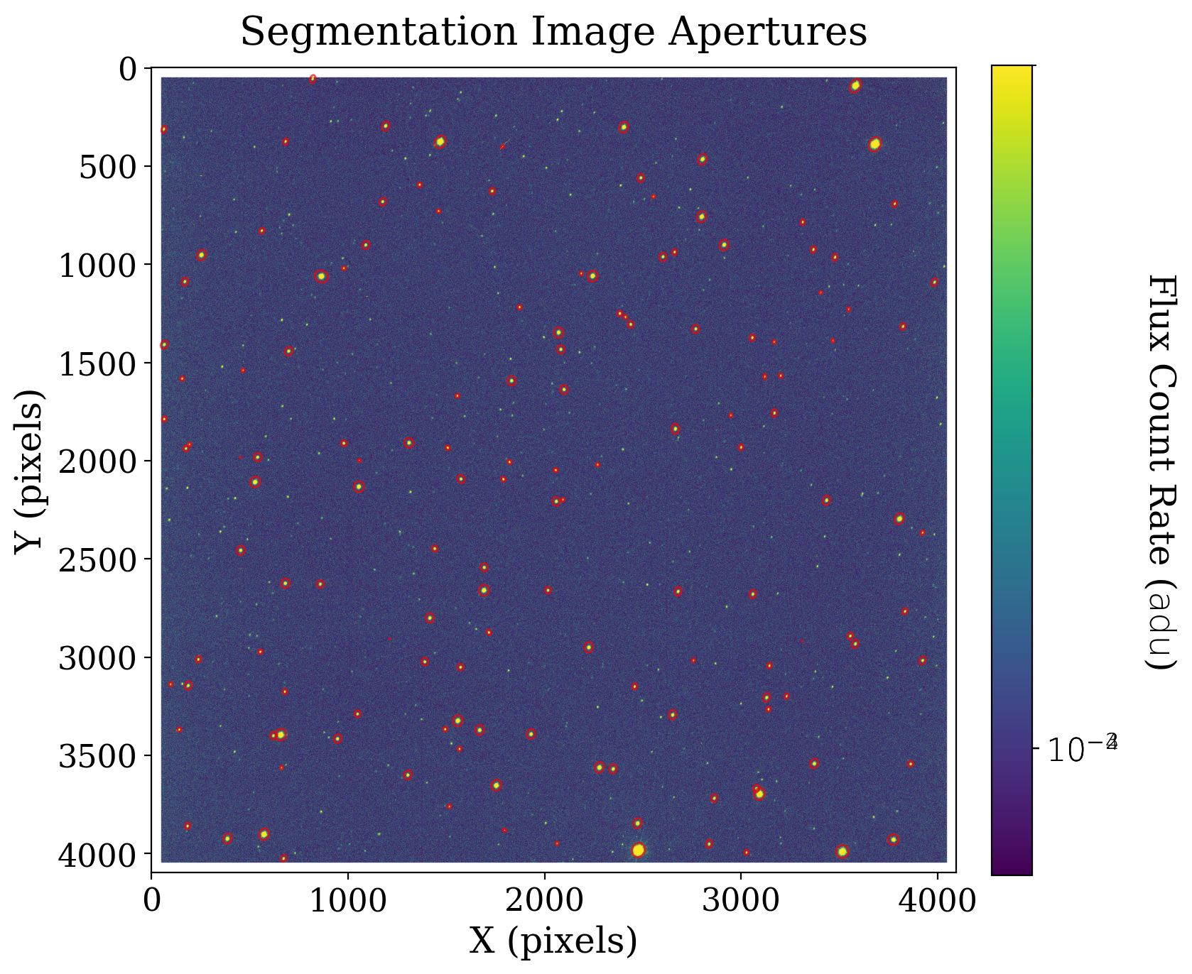
We can use this information to create isophotal ellipses for each identified source. These ellipses can also later be used as photometric apertures.

# Define the approximate isophotal extent
r = 8.  # pixels

# Create the apertures
apertures = []
for obj in catalog:
    position = (obj.xcentroid, obj.ycentroid)
    a = obj.semimajor_sigma.value * r
    b = obj.semiminor_sigma.value * r
    theta = obj.orientation
    apertures.append(EllipticalAperture(position, a, b, theta=theta))

8.4.3.1.1. Sources detected by image segmentation

All of the bright sources are detected by image segmentation.

# Set up the figure with subplots
fig, ax1 = plt.subplots(1, 1, figsize=(8, 8))

# Plot the data
fitsplot = ax1.imshow(np.ma.masked_where(ccd_2d_bkgdsub.mask, ccd_2d_bkgdsub),
                      norm=norm_image, cmap=cmap)

# Plot the apertures
for aperture in apertures:
    aperture.plot(color='red', lw=1, alpha=0.7, axes=ax1)

# Define the colorbar
cbar = plt.colorbar(fitsplot, fraction=0.046, pad=0.04, ticks=LogLocator())

def format_colorbar(bar):
    # Add minor tickmarks
    bar.ax.yaxis.set_minor_locator(LogLocator(subs=range(1, 10)))

    # Force the labels to be displayed as powers of ten and only at exact powers of ten
    bar.ax.set_yticks([1e-4, 1e-3, 1e-2])
    labels = [f'$10^{{{pow:.0f}}}$' for pow in np.log10(bar.ax.get_yticks())]
    bar.ax.set_yticklabels(labels)

format_colorbar(cbar)

# Define labels
cbar.set_label(r'Flux Count Rate ({})'.format(ccd_image.unit.to_string('latex')),
               rotation=270, labelpad=30)
ax1.set_xlabel('X (pixels)')
ax1.set_ylabel('Y (pixels)')
ax1.set_title('Segmentation Image Apertures');

8.4.3.2. Comparison with other detection methods

We rerun peak finding and star finding on this image so that we can compare the methods

with warnings.catch_warnings(action="ignore"):
    sources_findpeaks = find_peaks(ccd_2d_bkgdsub.data - median, mask=ccd_2d_bkgdsub.mask,
                                   threshold=threshold, box_size=29,
                                   centroid_func=centroid_2dg)

# Add an ID column to the find_peaks result
sources_findpeaks["source_id"] = np.arange(len(sources_findpeaks))

daofind = DAOStarFinder(fwhm=1.5 * fwhm, threshold=threshold)
sources_dao = daofind(np.ma.masked_where(ccd_image.mask, ccd_image), mask=ccd_2d_bkgdsub.mask)

# Set up the figure with subplots
fig, ax1 = plt.subplots(1, 1, figsize=(8, 8))

# Plot the data
fitsplot = ax1.imshow(np.ma.masked_where(ccd_2d_bkgdsub.mask, ccd_2d_bkgdsub),
                      norm=norm_image, cmap=cmap)

# Plot the apertures
apertures[0].plot(color='red', lw=2, alpha=1, axes=ax1, label="Image segmentation")
for aperture in apertures[1:]:
    aperture.plot(color='red', lw=2, alpha=1, axes=ax1)

# Add find_peaks sources
ax1.scatter(sources_findpeaks["x_centroid"], sources_findpeaks["y_centroid"], 
            marker="x", color="orange", s=200, lw=2, alpha=0.7, label="find_peaks")

# Add find_peaks sources
ax1.scatter(sources_dao["xcentroid"], sources_dao["ycentroid"], 
            marker="s", facecolor="none", edgecolor="cyan", s=200, alpha=0.5, label="DAOFind")

top = 1125
left = 2350
cutout_size = 500

# ax1.set_xlim(left, left + cutout_size)
# ax1.set_ylim(top, top + cutout_size)

ax1.legend(ncols=3, loc='lower center', bbox_to_anchor=(0.5, 1))

ax1.set_title('Source detection method comparison', y=1.05);

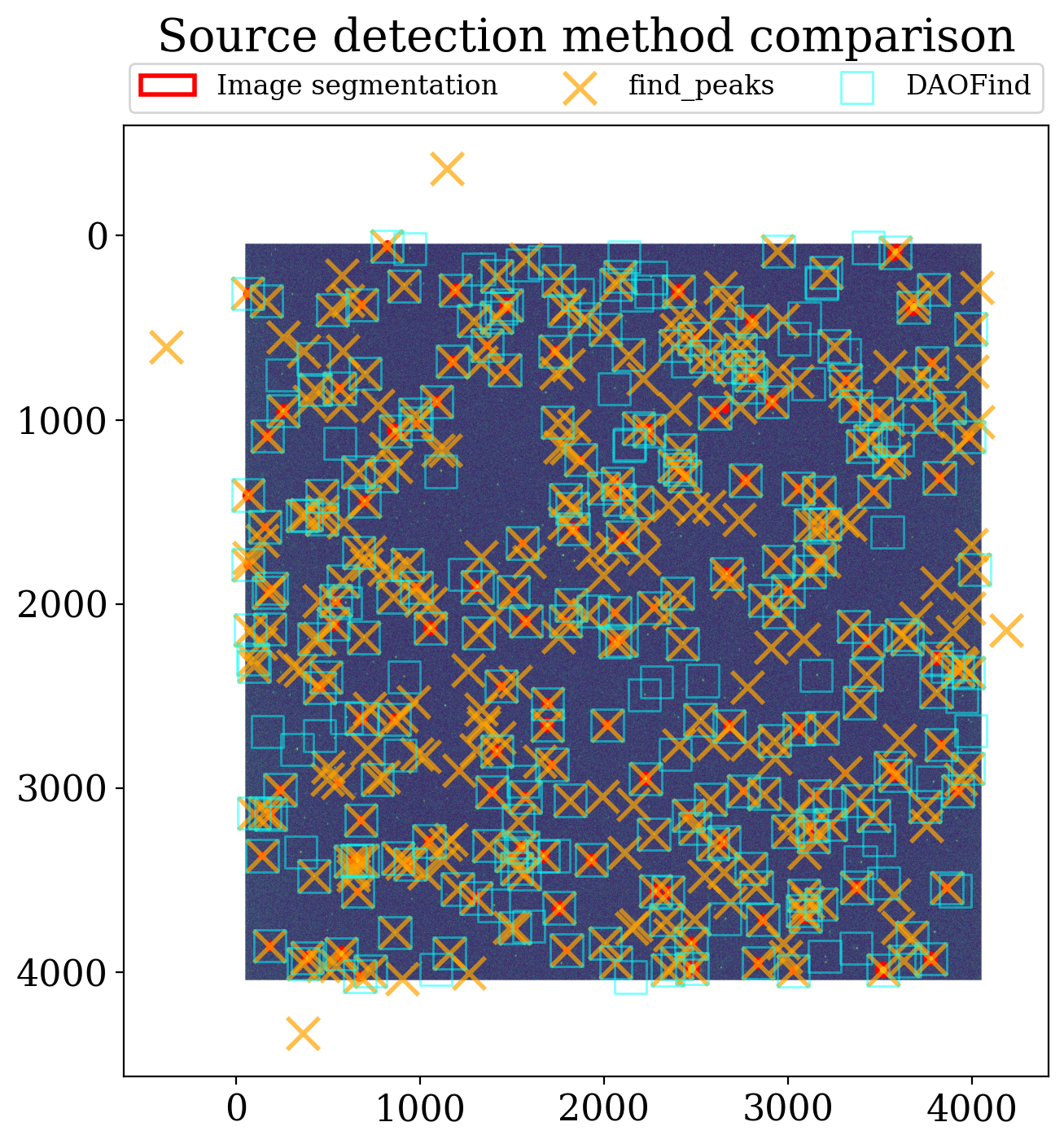
8.4.3.3. Summary

The image above nicely captures the differences between the source detection methods we have discussed. DAOStarFinder does an excellent job detecting the star-like sources in the image. find_peaks detects almost everything that DAOStarFinder does but also has many false identifications. Image segmentation does an excellent job detecting sources though it misses some of the fainter sources found by DAOStarFinder. This could likely be fixed by adjusting the settings for image segmentation.

The choice of source detection method in a case like may come down to whether you have additional constraints you want to impose. Recall that the IRAFStarFinder allows to to provide a minimum separation of sources, for example. For performing aperture photometry that is useful since there is no way to separate sources with that technique.