8.2.3. Source detection in a stellar image

8.2.3.1. Which data are used in this notebook?

The image in this notebook is of the field of the star TIC 125489084 on a night when the moon was nearly full. The moonlight caused a smooth gradient across the background of the image.

As discussed in the section about background subtraction with this image, the best way to remove the background in this case is to use photutils to construct a 2D model of the background.

As we will see in a moment, DAOStarFinder does a good job identifying most of the sources in the image, since all of the sources are stars.

8.2.3.2. Import necessary packages

First, let’s import packages that we will use to perform arithmetic functions and visualize data:

import numpy as np

from astropy.io import fits
from astropy.nddata import CCDData
import astropy.units as u
from astropy.stats import sigma_clipped_stats, SigmaClip
from astropy.visualization import ImageNormalize, LogStretch, AsymmetricPercentileInterval
import matplotlib.pyplot as plt
from matplotlib.ticker import LogLocator

from photutils.aperture import CircularAperture
from photutils.background import Background2D, MeanBackground
from photutils.detection import DAOStarFinder
from photutils.segmentation import detect_threshold, detect_sources
from photutils.utils import circular_footprint

# Show plots in the notebook
%matplotlib inline

Let’s also define some matplotlib parameters, such as title font size and the dpi, to make sure our plots look nice. To make it quick, we’ll do this by loading a style file shared with the other photutils tutorials into pyplot. We will use this style file for all the notebook tutorials. (See here to learn more about customizing matplotlib.)

plt.style.use('../photutils_notebook_style.mplstyle')

8.2.3.3. Load the data

Throughout this notebook, we are going to store our images in Python using a CCDData object (see Astropy documentation), which contains a numpy array in addition to metadata such as uncertainty, masks, and units.

ccd_image = CCDData.read('TIC_125489084.01-S001-R055-C001-ip.fit.bz2')
data = ccd_image.data
header = ccd_image.header

WARNING: FITSFixedWarning: RADECSYS= 'FK5 ' / Equatorial coordinate system 
the RADECSYS keyword is deprecated, use RADESYSa. [astropy.wcs.wcs]

8.2.3.4. Perform 2-D background estimation and subtraction

For more discussion of the choices here, see background subtraction with this image. The next couple of cells calculate the background and subtract it, and then display the background-subtracted data.

sigma_clip = SigmaClip(sigma=3., maxiters=5)
bkg_estimator = MeanBackground()
bkg = Background2D(ccd_image, box_size=200, filter_size=(9, 9), mask=ccd_image.mask,
                   sigma_clip=sigma_clip, bkg_estimator=bkg_estimator)
# Calculate the 2D background subtraction, maintaining metadata, unit, and mask
ccd_2d_bkgdsub = ccd_image.subtract(bkg.background)

# Set up the figure with subplots
fig, ax1 = plt.subplots(1, 1, figsize=(10, 10), sharey=True)
plt.tight_layout()


ax1.set_ylabel('Y (pixels)')
ax1.set_xlabel('X (pixels)')

# Plot the 2D-subtracted data
norm_image_sub = ImageNormalize(ccd_2d_bkgdsub, interval=AsymmetricPercentileInterval(30, 99.5))

fitsplot = ax1.imshow(np.ma.masked_where(ccd_2d_bkgdsub.mask, ccd_2d_bkgdsub), norm=norm_image_sub)
ax1.set_title('2D Background-Subtracted Data')

# Define the colorbar...
cbar_ax = fig.add_axes([1, 0.09, 0.03, 0.87])

cbar = fig.colorbar(fitsplot, cbar_ax)

cbar.set_label(r'Counts ({})'.format(ccd_image.unit.to_string('latex')),
               rotation=270, labelpad=30)

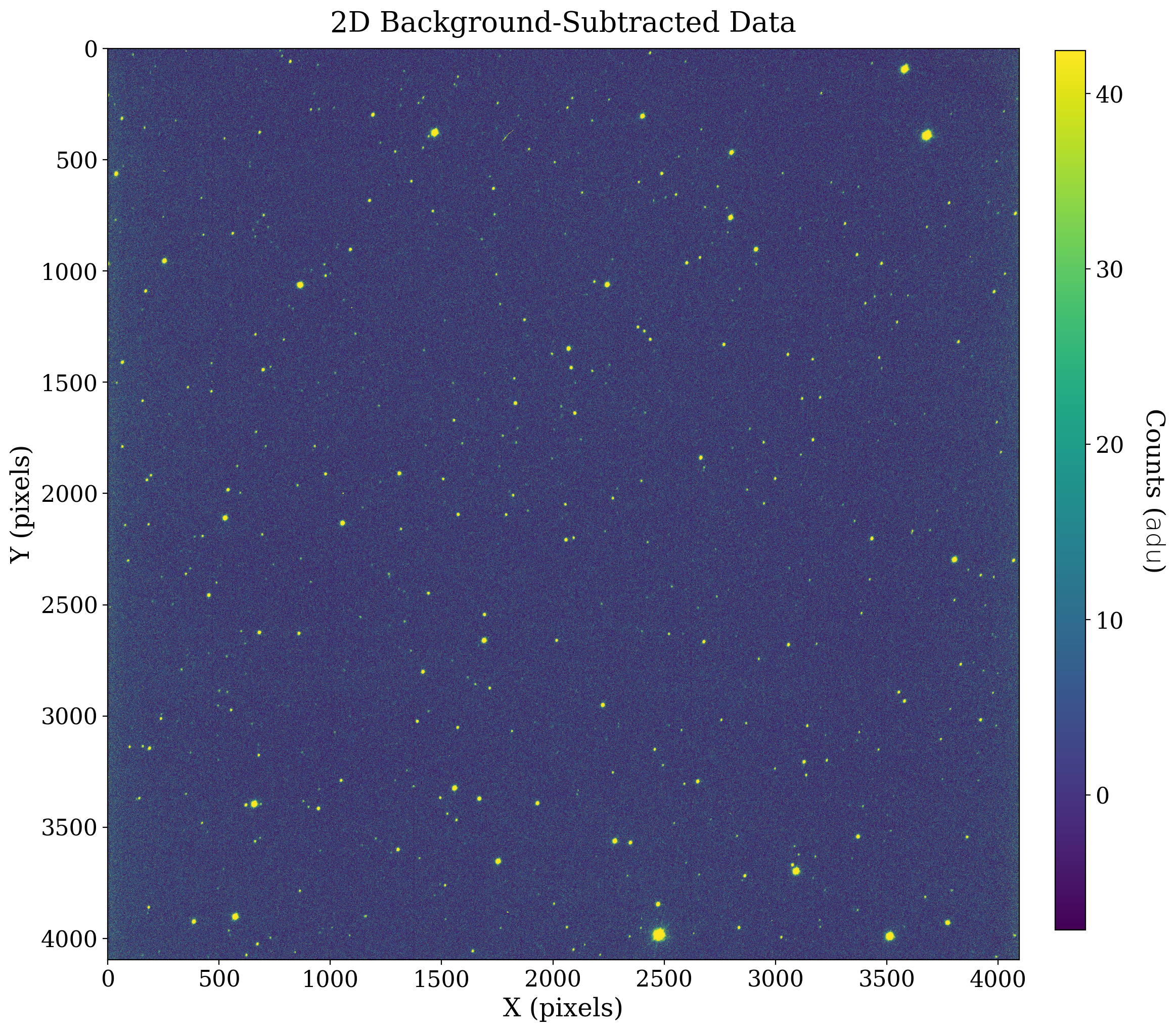
Note that after subtraction the background of the image looks fairly uniform.

8.2.3.5. Source detection

We will use the DAOStarFinder to detect the sources in this image. The typical full width half maximum (FWHM) of the stars in the image is about 6.2 pixels. For the detection threshold, we will use 5 times the standard deviation of the sigma-clipped image.

In addition, we’ll mask out the area within 50 pixels of the edge of the image, where the stars are often elongated on this camera.

mean, median, std = sigma_clipped_stats(ccd_2d_bkgdsub.data, sigma=3, maxiters=5)

# Create a mask array
mask = np.zeros_like(ccd_2d_bkgdsub, dtype=bool)

# Set the mask for a border of 50 pixels around the image
mask[:50, :] = mask[-50:, :] = mask[:, :50] = mask[:, -50:] = 1.0

# Create the star finder
fwhm = 6.2
daofinder = DAOStarFinder(threshold=5 * std, fwhm=fwhm)

# Find the sources, excluding the masked region

sources = daofinder(ccd_2d_bkgdsub.data, mask=mask)
print(f"Found {len(sources)} sources in the image")

Found 266 sources in the image

8.2.3.5.1. Source locations

There were 266 sources found in the image. Their locations are shown below, overlaid on the image itself.

positions = np.transpose((sources['xcentroid'], sources['ycentroid']))
apertures = CircularAperture(positions, r=3 * fwhm)

plt.figure(figsize=(10, 10))
plt.imshow(np.ma.masked_where(ccd_2d_bkgdsub.mask, ccd_2d_bkgdsub), norm=norm_image_sub)
apertures.plot(color="red");

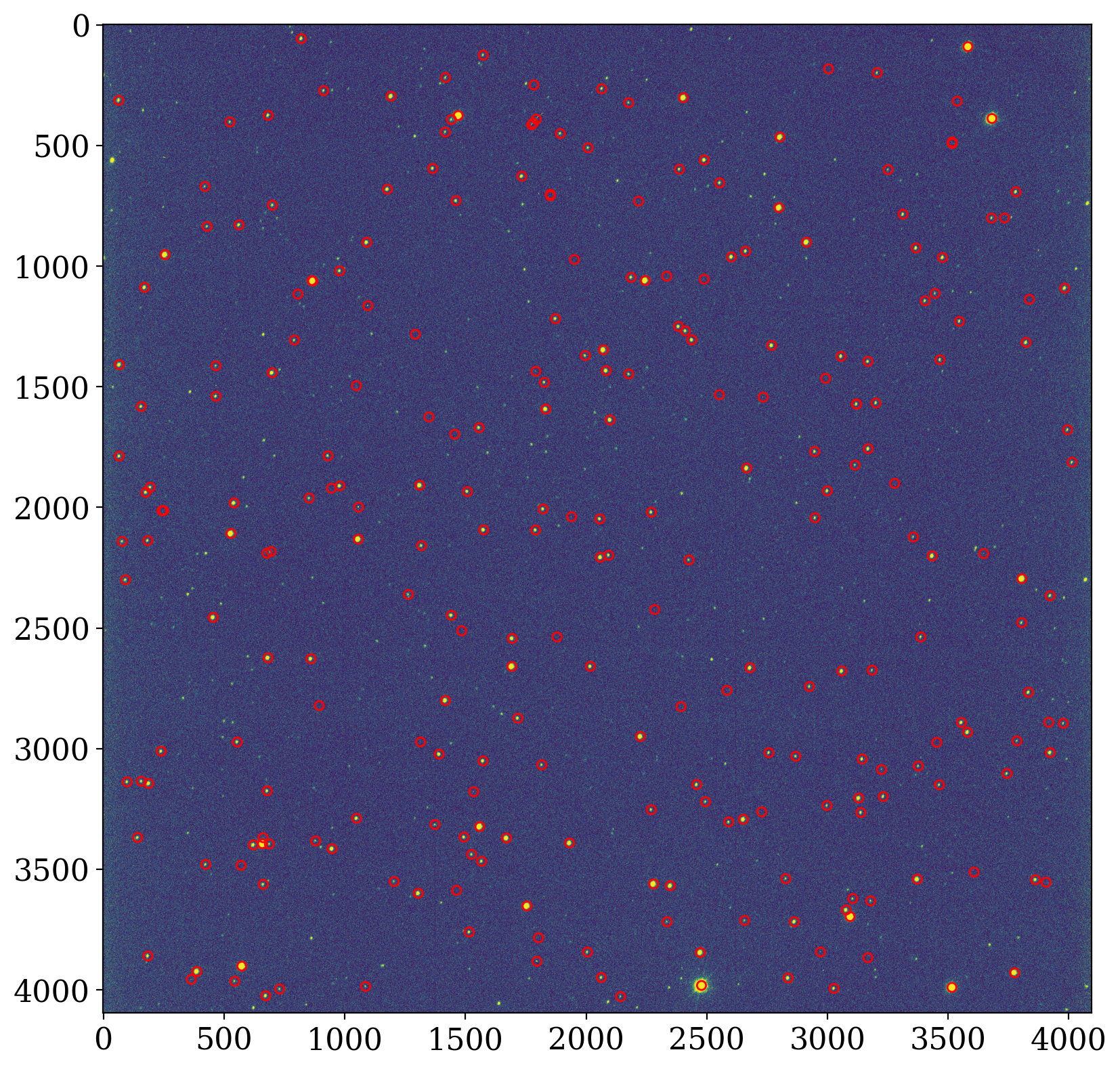
This seems to have a reasonably good job finding stars in the image. Many of the fainter stars were not detected, though.

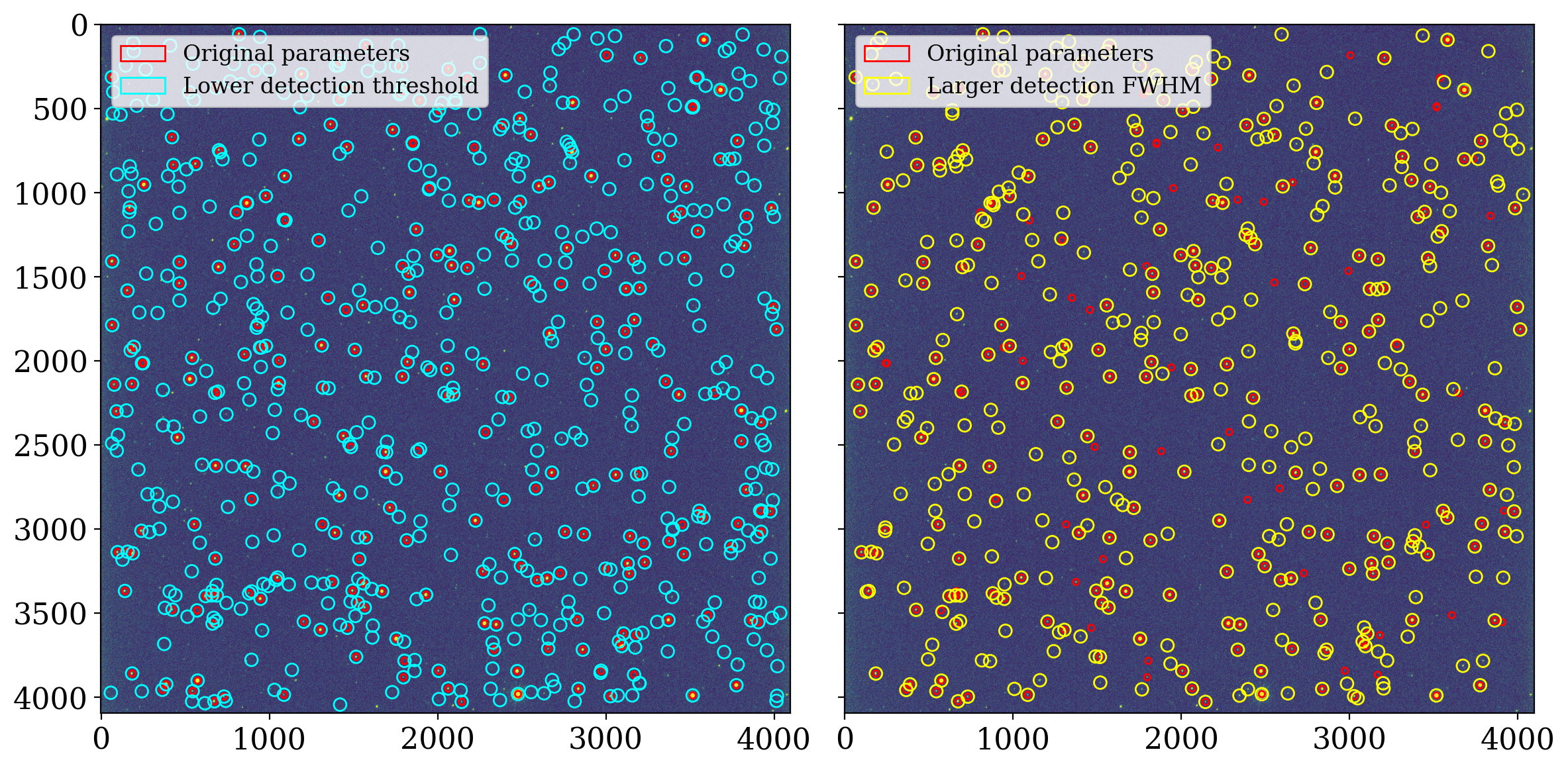
8.2.3.5.2. Improving the accuracy of source detection

You might at first be tempted to lower the threshold for detection. It turns out that that will report many more detections, but many of them will not actually be stars. A more effective approach is to increase the FWHM used by DAOStarFinder instead, to something like 1.5 or 2 × the FWHM of the stars in the image.

Below is a comparison of these two approaches with the source detection we did above.

daofinder_fainter = DAOStarFinder(threshold=4 * std, fwhm=fwhm)

daofinder_bigger_fwhm = DAOStarFinder(threshold=5 * std, fwhm=2 * fwhm)

sources_fainter = daofinder_fainter(ccd_2d_bkgdsub.data, mask=mask)
sources_bigger_fwhm = daofinder_bigger_fwhm(ccd_2d_bkgdsub.data, mask=mask)

def plot_with_label(apertures, label_text="", **kwd):
    apertures[0].plot(label=label_text, **kwd)
    apertures[1:].plot(**kwd)

fig, axes = plt.subplot_mosaic([['lower threshold', 'bigger fwhm']], figsize=(12, 6), sharey=True, tight_layout=True)


for ax in axes.values():
    ax.imshow(np.ma.masked_where(ccd_2d_bkgdsub.mask, ccd_2d_bkgdsub), norm=norm_image_sub)
    plot_with_label(apertures, color="red", label_text="Original parameters", ax=ax)

positions_fainter = np.transpose((sources_fainter['xcentroid'], sources_fainter['ycentroid']))
apertures_fainter = CircularAperture(positions_fainter, r=6 * fwhm)
plot_with_label(apertures_fainter, label_text="Lower detection threshold", color="cyan", ax=axes['lower threshold'])

positions_bigger_fwhm = np.transpose((sources_bigger_fwhm['xcentroid'], sources_bigger_fwhm['ycentroid']))
apertures_bigger_fwhm = CircularAperture(positions_bigger_fwhm, r=6 * fwhm)
plot_with_label(apertures_bigger_fwhm, label_text="Larger detection FWHM", color="yellow", ax=axes['bigger fwhm'])

for ax in axes.values():
    ax.legend(loc="upper left")

8.2.3.6. Summary

The DAOStarFinder works very well for detecting sources in an image, though the parameters may need to be tuned a bit for your images. The previous notebook compared DAOStarFinder and IRAFStarFinder. One of the important differences is that IRAFStarFinder allows you to impoose a minimum separation of sources, which may be important in some situations.