8.1.1. Overview of background subtraction using simulated data

The first step in detecting sources is to remove any background from the image. This notebook walks through a couple of ways to do that: using a single value for the background or constructing a two dimensional background image.

The imports for this notebook are in the cell below.

import numpy as np

%matplotlib inline
import matplotlib.pyplot as plt

from photutils.background import Background2D, MeanBackground, MADStdBackgroundRMS
from photutils.datasets import make_100gaussians_image
from photutils.segmentation import detect_threshold, detect_sources
from photutils.utils import circular_footprint

from astropy.visualization import SqrtStretch
from astropy.visualization.mpl_normalize import ImageNormalize
from astropy.visualization import hist
from astropy.stats import sigma_clipped_stats, SigmaClip

8.1.1.1. Simple approach: median or other scalar estimator of background

The simplest way to estimate the background is with a single number, perhaps the mean or median of the data. The problem with that approach is that the distribution of pixel value in an astronomical image is not symmetric. Most of the pixels have values near zero while a small number have significantly higher values.

The photutils documentation on scalar background and noise estimation walk through this step-by-step, demonstrating the result you get with a variety of background estimators.

The upshot is that the best estimate of the background is obtained by first masking the sources in the image and then sigma clipping the unmasked parts of the data. The mean and median of the unmasked parts of the image give almost exactly the same value, and standard deviation recovered from the data matches that of the input.

8.1.1.1.1. Pixel distribution in simulated image

We begin by constructing a histogram of pixel values in a sample image. The code below illustrates a few useful things from astropy and photutils:

• photutils comes with useful simulated images.

• astropy comes with a histogram function that will automatically bin the data in a way that brings out features in your data that uniform-width bins might miss.

• astropy has several stretches and normalizations to bring out features in astronomical images.

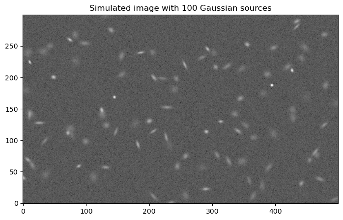
The simulated image we will work with in this section is below.

data = make_100gaussians_image()

# Create an image stretch that will be applied when we display the image.
norm = ImageNormalize(stretch=SqrtStretch())

plt.figure(figsize=(10, 5))
plt.imshow(data, norm=norm, origin='lower', cmap='Greys_r')
plt.title("Simulated image with 100 Gaussian sources")

Text(0.5, 1.0, 'Simulated image with 100 Gaussian sources')

Next we plot a histogram of the pixel values in the image. As suggested at the beginning of this section, the distribution is not symmetric.

plt.figure(figsize=(10, 5))

# IMPORTANT NOTE: flattening the data to one dimension vastly reduces the
# time it takes to histogram the data.

h, bins, patches = hist(data.flatten(), bins='freedman', log=True,
                        alpha=0.5, label='Pixel values')
plt.xlabel('Pixel value')
plt.ylabel('Number of pixels')
plt.title("Histogram of pixel values")
# The semi-colon suppresses a display of the grid object representation
plt.grid();

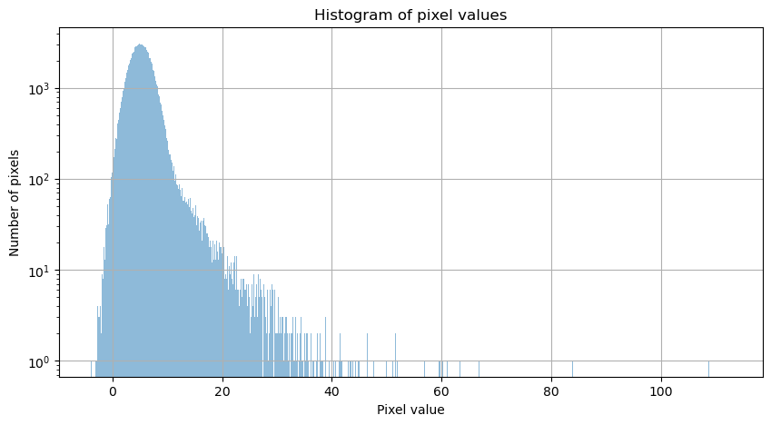
There are a couple of things to note about this distribution.

The bulk of the pixel values are noise. The function make_100gaussians_image adds a background with a Gaussian distribution centered at 5 with a standard deviation of 2. The long tail at higher pixel values are from the sources in the image.

8.1.1.1.2. Estimating the background value

The plot below shows the result of several ways of estimating the background from the data:

• mean of all of the pixels

• median of all of the values

• a sigma-clipped median of all of the values.

None of these straightforward estimates give a good measure of the true background level, which is indicated by the green line.

plt.figure(figsize=(10, 5))
hist(data.flatten(), bins='freedman', log=True,
                        alpha=0.5, label='Pixel values')
plt.xlim(0, 10)

true_mean = 5
avg_all_pixels = data.mean()
median_all_pixels = np.median(data)
plt.axvline(true_mean, label='True mean of background', color='green')
plt.axvline(avg_all_pixels, label='Mean of all values', color='red')
plt.axvline(median_all_pixels, label='Median of all values', color='cyan')

# Try sigma clipping
clipped_mean, clipped_med, clipped_std  = sigma_clipped_stats(data, sigma=3)

# Add line to chart
plt.axvline(clipped_med, label='Sigma-clipped median', color='yellow')
plt.xlabel('Pixel value')
plt.ylabel('Number of pixels')
plt.title("Methods of estimating background value")
plt.legend();

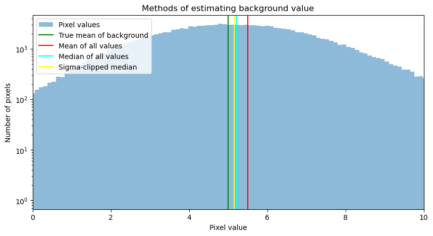
None of the estimates above do a particularly good job of estimating the true background level. They also do not do a great job of estimating the error or noise in that background; the input value was 2, but the value produced by sigma clipping is 5% larger:

clipped_std

2.094237385960309

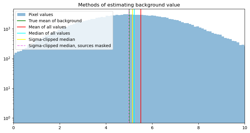
8.1.1.1.3. Best approach for single value

The best approach to deriving a single value to use for background is to first mask the sources. There are a few steps to doing that.

First, define the sigma clip parameters for deticting the threshold for sources

sigma_clip = SigmaClip(sigma=3.0, maxiters=10)

Next, find pixels more that 2\(\sigma\) above the background using detect_threshold.

threshold = detect_threshold(data, nsigma=2.0, sigma_clip=sigma_clip)

These pixels may be isolated or disconnected. The function detect_sources creates a segmentation image, in which only connected sets of npixels or more pixels are identified as sources.

segment_img = detect_sources(data, threshold, npixels=10)

Finally, we use make_source_mask to create a mask that is True where there are sources. It masks out a circular region 10 pixels in size at each source.

footprint = circular_footprint(radius=10)

source_mask = segment_img.make_source_mask(footprint=footprint)

We now add the sigma-clipped median of just the pixels without a source in them.

mask_clip_mean, mask_clip_med, mask_clip_std  = sigma_clipped_stats(data, sigma=3, mask=source_mask)

plt.figure(figsize=(10, 5))
hist(data.flatten(), bins='freedman', log=True,
                        alpha=0.5, label='Pixel values')
plt.xlim(0, 10)

plt.axvline(true_mean, label='True mean of background', color='green')
plt.axvline(avg_all_pixels, label='Mean of all values', color='red')
plt.axvline(median_all_pixels, label='Median of all values', color='cyan')
plt.axvline(clipped_med, label='Sigma-clipped median', color='yellow')
plt.axvline(mask_clip_med, label='Sigma-clipped median, sources masked',
            color='violet', linestyle='dashed')
plt.title("Methods of estimating background value")
plt.legend();

8.1.1.1.4. A caveat about the “best” approach

Note that the difference in value between the estimates of the background displayed above are not large. The one that is furthest off, the mean of all of the values, differs from the true value by half a count. Whether that is significant or not depends on what science you are trying to do, what sources of error are present in your data and how large they are, and how you will treat the data in later steps.

That is not to say there is anything wrong about the approach described in this section; it is just a reminder that the right choice for your data and science is not necessary what is described here as the best choice.

8.1.1.2. Two dimensional background

If the background is not uniform (as happens, for example, on a night with moonlight) then using a single value to represent that background will not be effective. Instead, one constructs a background array. It is constructed by breaking the image into pieces, calcuating a scalar background estimate as above, and building those back into a two-dimensional image.

To do this with photutils requires making a few choices:

• What should the mesh size be? This is the size, in pixels, of the chunks into which the image will be split for generating the background. It should be larger than the sources in the image, but small enough to represent variation in background across the image.

• How should the background in each mesh cell be calculated? The full suite of options is listed in the photutils documentation for 2D backgrounds. The example below uses the mean because the sources will be masked as in the scalar case. Other options include the median and SExtractorBackground for using the background method used by Source Extractor.

• Do you want to also estimate the noise in the background, i.e. the RMS of the background? Again, several options are available.

• How do you want the background image interpolated when it is scaled back up to the size of the input image? By default spline interpolation is used, but it can be changed.

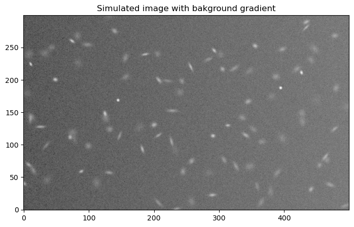
8.1.1.2.1. Add some background to the input image

As with the rest of the examples in this notebook, we closely follow the example from the photutils documentation. The gradient added here might resemble what you would ee on a moonlit night near the moon.

ny, nx = data.shape
y, x = np.mgrid[:ny, :nx]

gradient = x / 50.
gradient_median = np.median(gradient)
data2 = data + gradient

plt.figure(figsize=(10, 5))
plt.imshow(data2, norm=norm, origin='lower', cmap='Greys_r')
plt.title("Simulated image with bakground gradient");

8.1.1.2.2. Choose your options for constructing the background

For most of the choices in the list above, one creates an instance of the class corresponing to the choice.

# Choose sigma clip parameters

# Parameters below match those used in sigma_clipped_stats above. The
# default in photutils is sigma=3, iters=10; this default is used unless
# you override it as shown below.
sigma_clip = SigmaClip(sigma=3., maxiters=5)

# Choose your background calculation method
bg_estimator = MeanBackground()

# Choose your mesh size...ideally, an integer number of these fits across
# the image. Here we use a size such that 10 meshes fit across the image
# in each directory.
mesh_size = (ny // 10, nx // 10)

# Choose an estimator for the noise in the background (i.e. RMS). The
# default is to use standard deviation using StdBackgroundRMS. This
# example uses the median absolute deviation for the purposes of
# illustration.
bg_rms_estimator = MADStdBackgroundRMS()

# We could, in principle, specify an interpolator for going from the small
# mesh to the full size image. By not specifying that we get the default,
# which is a spline interpolation; photutils calls this BgZoom

# Finally, construct the background. Each of the choices above are fed into
# the initialization of the background object.
bgd = Background2D(data2, mesh_size,
                   sigma_clip=sigma_clip,
                   bkg_estimator=bg_estimator,
                   bkgrms_estimator=bg_rms_estimator,
                  )

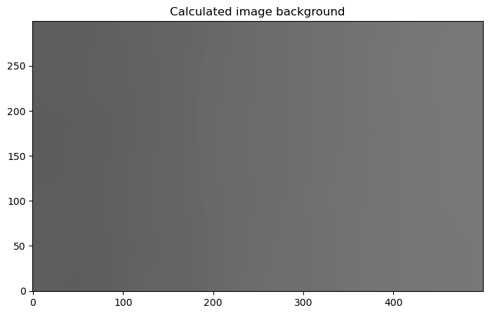
8.1.1.2.3. Display the background

Though this is not required, we may as well check to see whether the inferred background matches the gradient in the x-direction that we added to the image.

plt.figure(figsize=(10, 5))
plt.imshow(bgd.background, norm=norm, origin='lower', cmap='Greys_r')
plt.title("Calculated image background");

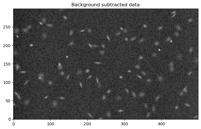
8.1.1.2.4. Check: compare background-subtracted data to expected values

If the background has been properly substracted, then the median of the subtracted image should be zero (if we mask out the sources) and the rms should be around 2, the value that was used to generate the Gaussian noise in make_100gaussians_image.

back_sub_data = data2 - bgd.background

sub_mean, sub_med, sub_std  = sigma_clipped_stats(back_sub_data, sigma=3)

print(f"Mean: {sub_mean}, Median: {sub_med}, Standard deviation: {sub_std}")

Mean: 0.007930618914160865, Median: -0.036326299505641924, Standard deviation: 2.115990478902112

8.1.1.2.5. Background-subtracted image

Finally, we display the background-subtracted image.

plt.figure(figsize=(10, 5))
plt.imshow(data2 - bgd.background, norm=norm, origin='lower', cmap='Greys_r')
plt.title('Background subtracted data')

Text(0.5, 1.0, 'Background subtracted data')

8.1.1.3. Summary

An image needs to be background-subtracted before you detect the sources in the image. That background can be represented by either a single number, e.g. the mean or median, or by a two-dimensional image. In both cases the best estimate of the background is obtained when sources are masked out before estimating the background. Though this means doing two rounds of source detection, one to estimate the background and one for the actual source detection, the method of finding sources used above is reasonably fast.

Next, we will look at how to do background estimation for a couple of actual science images to get a more nuanced understanding of the choices in background subtraction.