8.1.3. Removing a background gradient

8.1.3.1. Which data are used in this notebook?

The image in this notebook is of the field of the star TIC 125489084 on a night when the moon was nearly full. The moonlight caused a smooth gradient across the background of the image.

8.1.3.2. Import necessary packages

First, let’s import packages that we will use to perform arithmetic functions and visualize data:

import numpy as np

from astropy.io import fits
from astropy.nddata import CCDData
import astropy.units as u
from astropy.stats import sigma_clipped_stats, SigmaClip
from astropy.visualization import ImageNormalize, LogStretch, AsymmetricPercentileInterval
import matplotlib.pyplot as plt
from matplotlib.ticker import LogLocator

from photutils.segmentation import detect_threshold, detect_sources
from photutils.utils import circular_footprint

# Show plots in the notebook
%matplotlib inline

Let’s also define some matplotlib parameters, such as title font size and the dpi, to make sure our plots look nice. To make it quick, we’ll do this by loading a style file shared with the other photutils tutorials into pyplot. We will use this style file for all the notebook tutorials. (See here to learn more about customizing matplotlib.)

plt.style.use('../photutils_notebook_style.mplstyle')

8.1.3.3. Load the data

Throughout this notebook, we are going to store our images in Python using a CCDData object (see Astropy documentation), which contains a numpy array in addition to metadata such as uncertainty, masks, and units.

ccd_image = CCDData.read('TIC_125489084.01-S001-R055-C001-ip.fit.bz2')
data = ccd_image.data
header = ccd_image.header

WARNING: FITSFixedWarning: RADECSYS= 'FK5 ' / Equatorial coordinate system 
the RADECSYS keyword is deprecated, use RADESYSa. [astropy.wcs.wcs]

Let’s look at the data below. The image normalization we use here is one that is often convenient to use for images with stellar sources.

# Set up the figure with subplots
fig, ax1 = plt.subplots(1, 1, figsize=(8, 8))

# Set up the normalization and colormap
norm_image = ImageNormalize(ccd_image, interval=AsymmetricPercentileInterval(30, 99.5))
cmap = plt.get_cmap('viridis')

# Plot the data
fitsplot = ax1.imshow(np.ma.masked_where(ccd_image.mask, ccd_image),
                      norm=norm_image, cmap=cmap)

# Define the colorbar
cbar = plt.colorbar(fitsplot, fraction=0.046, pad=0.04)

# Define labels
cbar.set_label(r'Counts ({})'.format(ccd_image.unit.to_string('latex')),
               rotation=270, labelpad=30)
ax1.set_xlabel('X (pixels)')
ax1.set_ylabel('Y (pixels)');

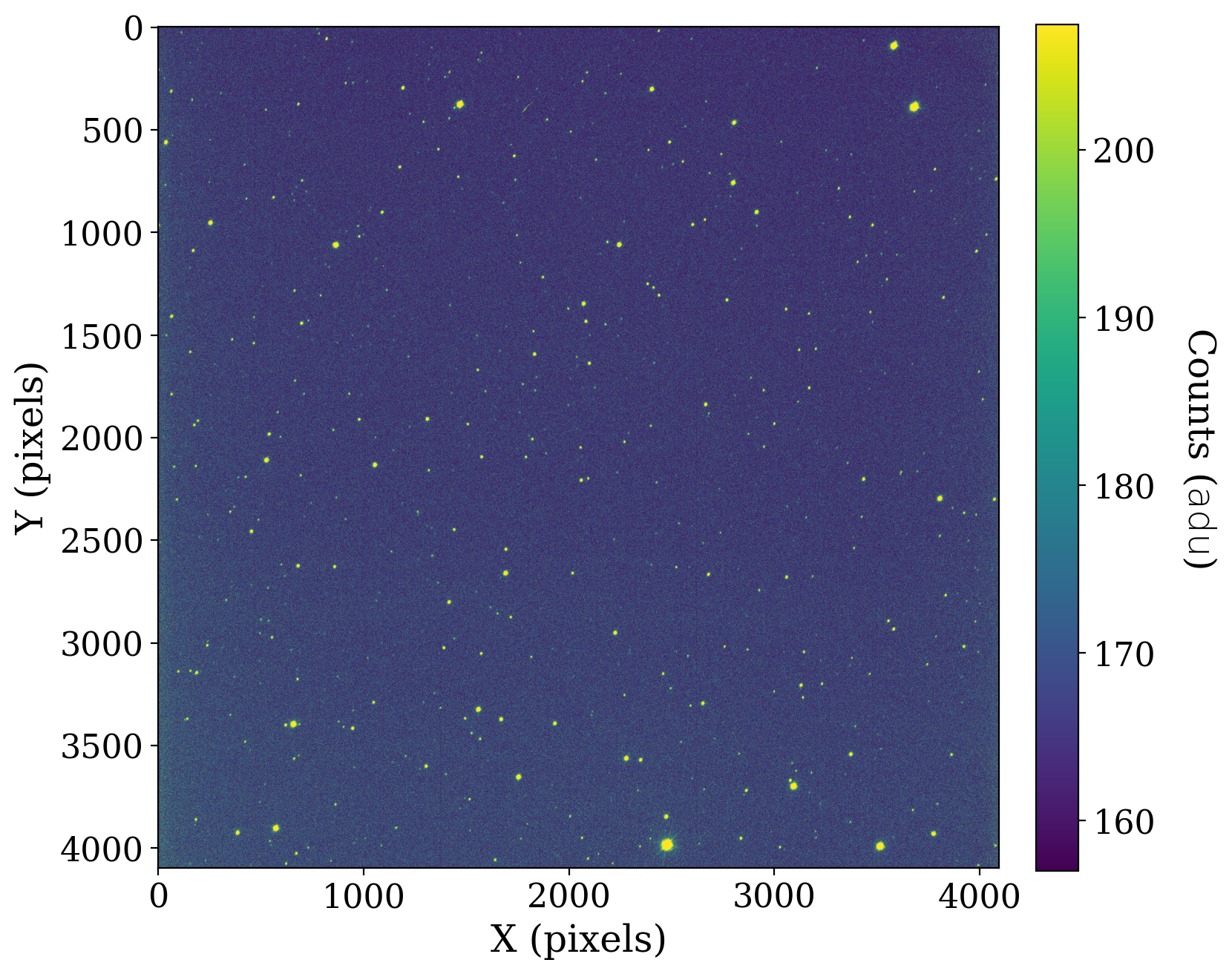
Unlike the XDF image, there are not any large sectregionsions of the image that contain no data. For consistency with the prior example, we create a mask for this image too.

ccd_image.mask = ccd_image.data == 0

8.1.3.4. Perform scalar background estimation

Now that the data are properly masked, we can calculate some basic statistical values to do a scalar estimation of the image background, as we did in the previous section.

8.1.3.4.1. Calculate scalar background value

Here we will calculate the mean, median, and mode of the dataset using sigma clipping. With sigma clipping, the data is iteratively clipped to exclude data points outside of a certain sigma (standard deviation), thus removing some of the noise from the data before determining statistical values.

In the first case we account for the mask while sigma clipping and in the second case we do not.

# Calculate statistics with masking
mean, median, std = sigma_clipped_stats(ccd_image.data, sigma=3.0, maxiters=5, mask=ccd_image.mask)

# Calculate statistics without masking
stats_nomask = sigma_clipped_stats(ccd_image.data, sigma=3.0, maxiters=5)

8.1.3.4.2. Calculate scalar background value without sigma clipping

Here we will calculate the mean, median, and mode of the dataset without using sigma clipping.

As above, we do this first taking into account the mask and then ignoring the mask.

mean_noclip_mask = np.mean(ccd_image.data[~ccd_image.mask])
median_noclip_mask = np.median(ccd_image.data[~ccd_image.mask])

mean_noclip_nomask = np.mean(ccd_image.data)
median_noclip_nomask = np.median(ccd_image.data)

8.1.3.4.3. Mask sources, then calculate scalar background

As discussed in [FILL IN LINK](FILL IN LINK), the most accurate estimate of the scalar background is obtained when the sources are masked first. The cell below does that procedure.

# Set up sigma clipping
sigma_clip = SigmaClip(sigma=3.0, maxiters=10)

threshold = detect_threshold(ccd_image.data, nsigma=2.0, sigma_clip=sigma_clip, mask=ccd_image.mask)
segment_img = detect_sources(ccd_image.data, threshold, npixels=10, mask=ccd_image.mask)
footprint = circular_footprint(radius=10)

# Make the source mask a circle of radius 10 around each detected source
source_mask = segment_img.make_source_mask(footprint=footprint)

# Compute the stats
source_mask_clip_mean, source_mask_clip_med, source_mask_clip_std  = sigma_clipped_stats(data, sigma=3, mask=source_mask)

What difference do sigma clipping and masking make in this case?

# Set up the figure with subplots
fig, [ax1, ax2] = plt.subplots(1, 2, figsize=(12, 4), sharey=True)

# Plot histograms of the data
flux_range = (100, 500)
ax1.hist(ccd_image.data[~ccd_image.mask], bins=500, range=flux_range)
ax2.hist(ccd_image.data[~ccd_image.mask], bins=500, range=flux_range)

# Plot lines for each kind of mean
ax1.axvline(mean, label='Non-data masked and Clipped', c='C1', ls='-.', ms=10, lw=3)
ax1.axvline(mean_noclip_mask, label='Masked', c='C2', lw=3)
ax1.axvline(stats_nomask[0], label='Clipped', c='C3', ls=':', lw=3)
ax1.axvline(source_mask_clip_mean, label='Sources masked and clipped', c='C4', lw=3)
ax1.axvline(mean_noclip_nomask, label='Neither', c='C5', ls='--', lw=3)

ax1.set_xlim(150, 220)
ax1.set_xlabel(r'Counts ({})'.format(ccd_image.unit.to_string('latex')), fontsize=14)
ax1.set_ylabel('Frequency', fontsize=14)
ax1.set_title('Mean pixel value', fontsize=16)

# Plot lines for each kind of median
# Note: use np.ma.median rather than np.median for masked arrays
ax2.axvline(median, label='Non-data masked and Clipped', c='C1', ls='-.', lw=3)
ax2.axvline(median_noclip_mask, label='Masked', c='C2', lw=3)
ax2.axvline(source_mask_clip_med, label='Sources masked and clipped', c='C4', lw=3)
ax2.axvline(stats_nomask[1], label='Clipped', c='C3', ls=':', lw=3)
ax2.axvline(median_noclip_nomask, label='Neither', c='C5', ls='--', lw=3)


ax2.set_xlim(160, 170)  # flux_range)
ax2.set_xlabel(r'Counts ({})'.format(ccd_image.unit.to_string('latex')), fontsize=14)
ax2.set_title('Median pixel value', fontsize=16)

# Add legend
ax1.legend(fontsize=11, loc='lower center', bbox_to_anchor=(1.1, -0.55), ncol=2, handlelength=6);

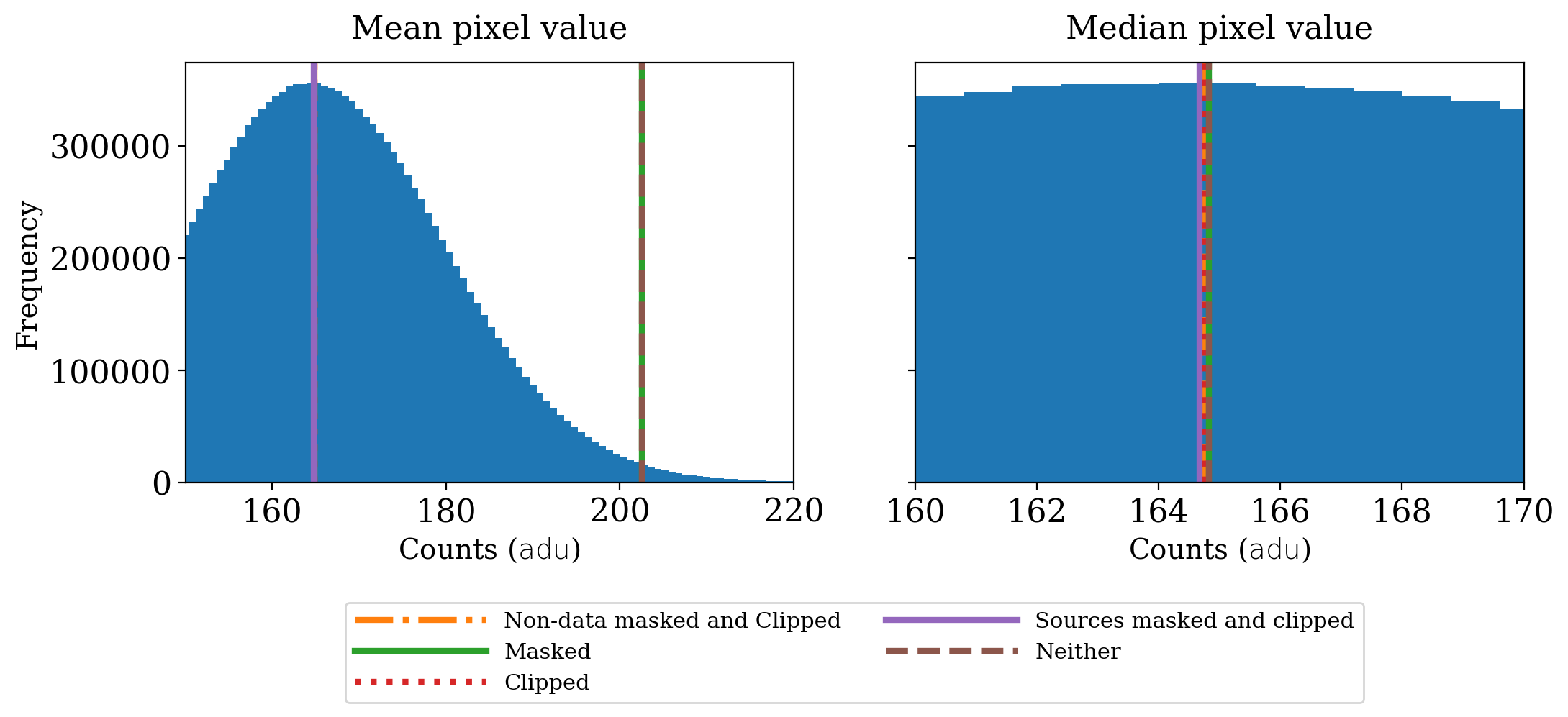
The contrast with the previous section that used XDF image is striking. In this case maskng makes no difference because there were no non-data areas to mask. Sigma clipping makes a much larger difference than in the XDF case because of the presence of a number of relatively bright stars in this image.

Once sigma clipping has been done it makes little difference whether sources are also masked.

The median value of the image is essentially the same no matter how it is calculated. Though the stars that are present are bright, they are a small fraction of the image.

8.1.3.4.4. Subtract scalar background value

We subtract the mean value of the scalar background below then discuss the resulting image.

# Calculate the scalar background subtraction, maintaining metadata, unit, and mask
ccd_scalar_bkgdsub = ccd_image.subtract(mean * u.adu)

# Set up the figure with subplots
fig, [ax1, ax2] = plt.subplots(1, 2, figsize=(12, 6), sharey=True)
plt.tight_layout()

# Plot the original data
fitsplot = ax1.imshow(np.ma.masked_where(ccd_image.mask, ccd_image), norm=norm_image)
ax1.set_xlabel('X (pixels)')
ax1.set_ylabel('Y (pixels)')
ax1.set_title('Original Data')

# Plot the subtracted data
fitsplot = ax2.imshow(ccd_scalar_bkgdsub, norm=norm_image)
ax2.set_xlabel('X (pixels)')
ax2.set_title('Scalar Background-Subtracted Data')

# Define the colorbar...
cbar_ax = fig.add_axes([1, 0.09, 0.03, 0.87])

cbar = fig.colorbar(fitsplot, cbar_ax)

cbar.set_label(r'Flux Count Rate ({})'.format(ccd_image.unit.to_string('latex')),
               rotation=270, labelpad=30)

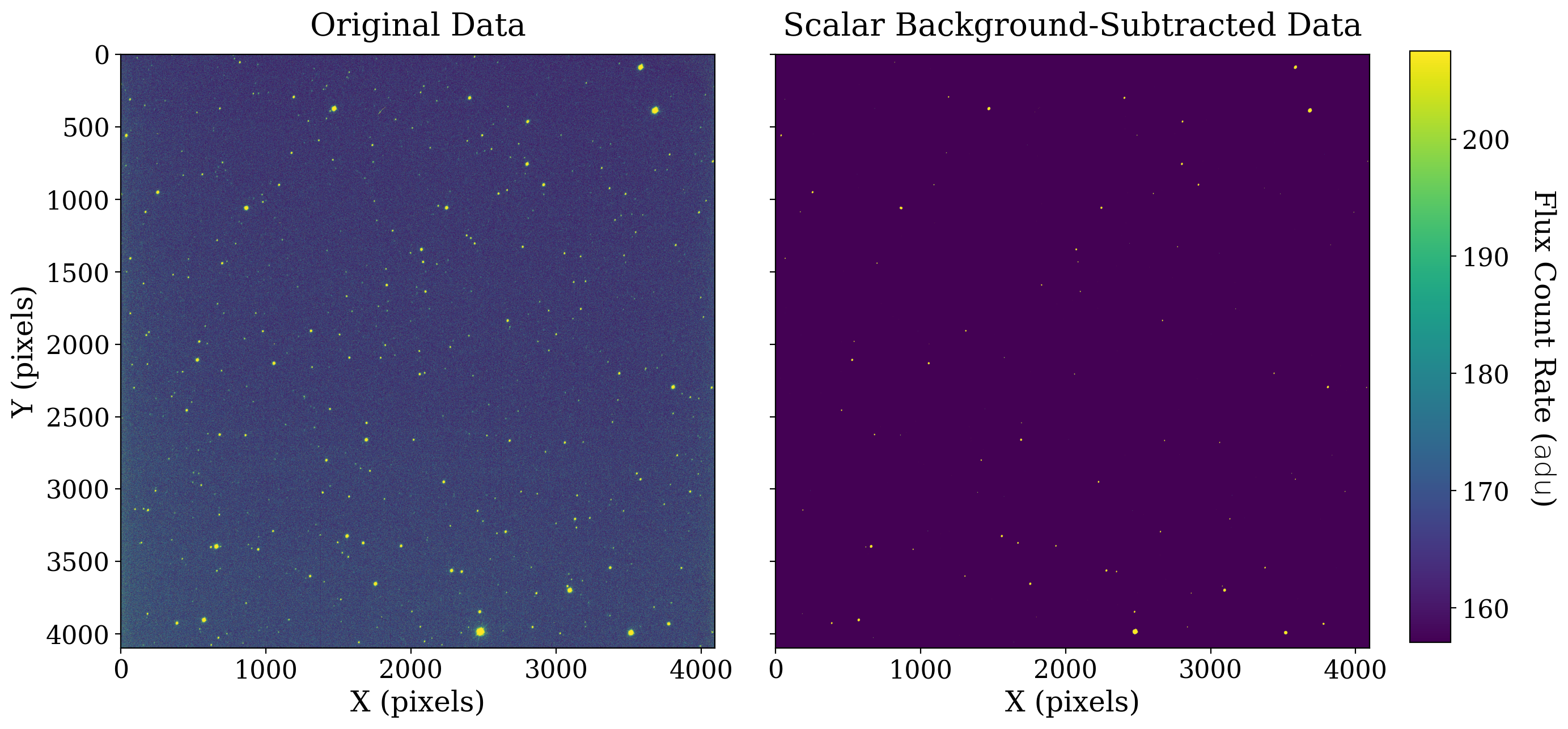
The result here may look surprising at first: background subtraction seems to have made everything much fainter. That is an artifact of using the same image normalization for both images even though the range of their data values is now very different.

In the image on the left, the average data value is roughly 165 adu. In the image on the right, the average value is roughly 0 adu by design, since we subtracted the mean of the first image from every pixel.

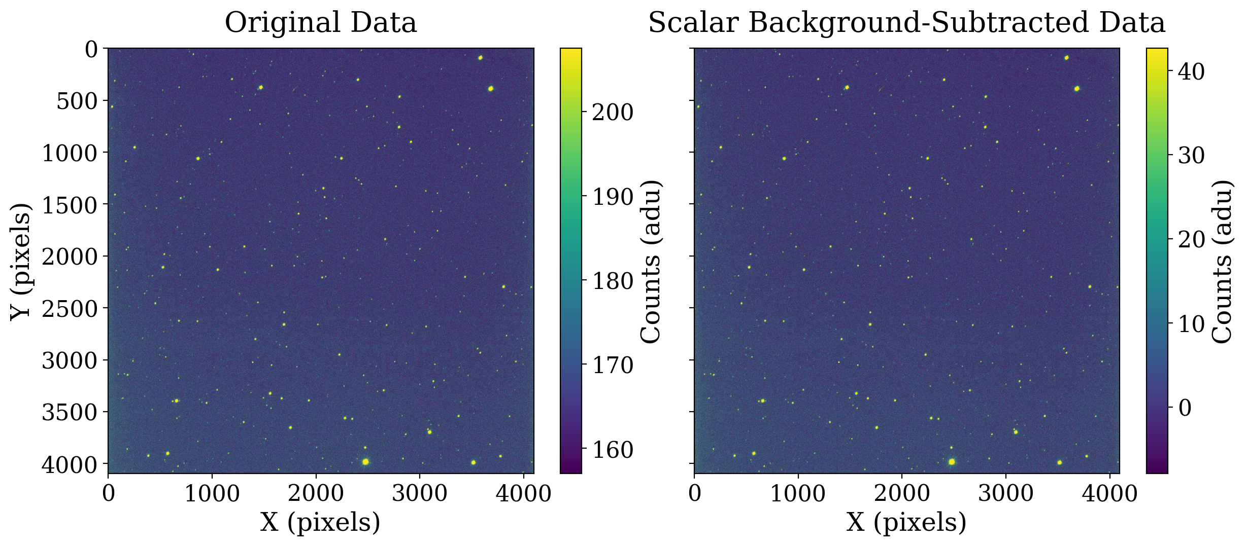
If we redo the plot but use a different image normalization for each it becomes clearer that the scalar background subtraction has one effect: moving the mean pixel value in the image.

# Set up the figure with subplots
fig, [ax1, ax2] = plt.subplots(1, 2, figsize=(12, 6), sharey=True)
plt.tight_layout()

# Plot the original data
original_image = ax1.imshow(np.ma.masked_where(ccd_image.mask, ccd_image), norm=norm_image)
ax1.set_xlabel('X (pixels)')
ax1.set_ylabel('Y (pixels)')
ax1.set_title('Original Data')
cb_orig = fig.colorbar(original_image, ax=ax1, shrink=0.8)
cb_orig.set_label(f'Counts ({ccd_image.unit})')

# Plot the subtracted data on its own color scale
norm_image_sub = ImageNormalize(ccd_scalar_bkgdsub, interval=AsymmetricPercentileInterval(30, 99.5))

subtracted_image = ax2.imshow(ccd_scalar_bkgdsub, norm=norm_image_sub)
ax2.set_xlabel('X (pixels)')
ax2.set_title('Scalar Background-Subtracted Data')
cb_sub = fig.colorbar(subtracted_image, ax=ax2, shrink=0.8)
cb_sub.set_label(f'Counts ({ccd_image.unit})')

8.1.3.5. Perform 2-D background estimation

The Background2D class in photutils allows users to model 2-dimensional backgrounds, by calculating the mean or median in small boxes, and smoothing these boxes to reconstruct a continuous 2D background. As in the previous notebook, we will use the MeanBackground estimator.

Here we expect that the background image will be useful since there is clearly a gradient in the image.

from photutils.background import Background2D, MeanBackground

sigma_clip = SigmaClip(sigma=3., maxiters=5)
bkg_estimator = MeanBackground()
bkg = Background2D(ccd_image, box_size=200, filter_size=(9, 9), mask=ccd_image.mask,
                   sigma_clip=sigma_clip, bkg_estimator=bkg_estimator)

# Set up the figure with subplots
fig, ax1 = plt.subplots(1, 1, figsize=(8, 8))

# Plot the background
fitsplot = ax1.imshow(np.ma.masked_where(ccd_image.mask, bkg.background.data), norm=norm_image)

# Define the colorbar
cbar = plt.colorbar(fitsplot, fraction=0.046, pad=0.04)

# Define labels
cbar.set_label(r'Flux Count Rate ({})'.format(ccd_image.unit.to_string('latex')),
               rotation=270, labelpad=30)
ax1.set_xlabel('X (pixels)')
ax1.set_ylabel('Y (pixels)')
ax1.set_title('2D Estimated Background');

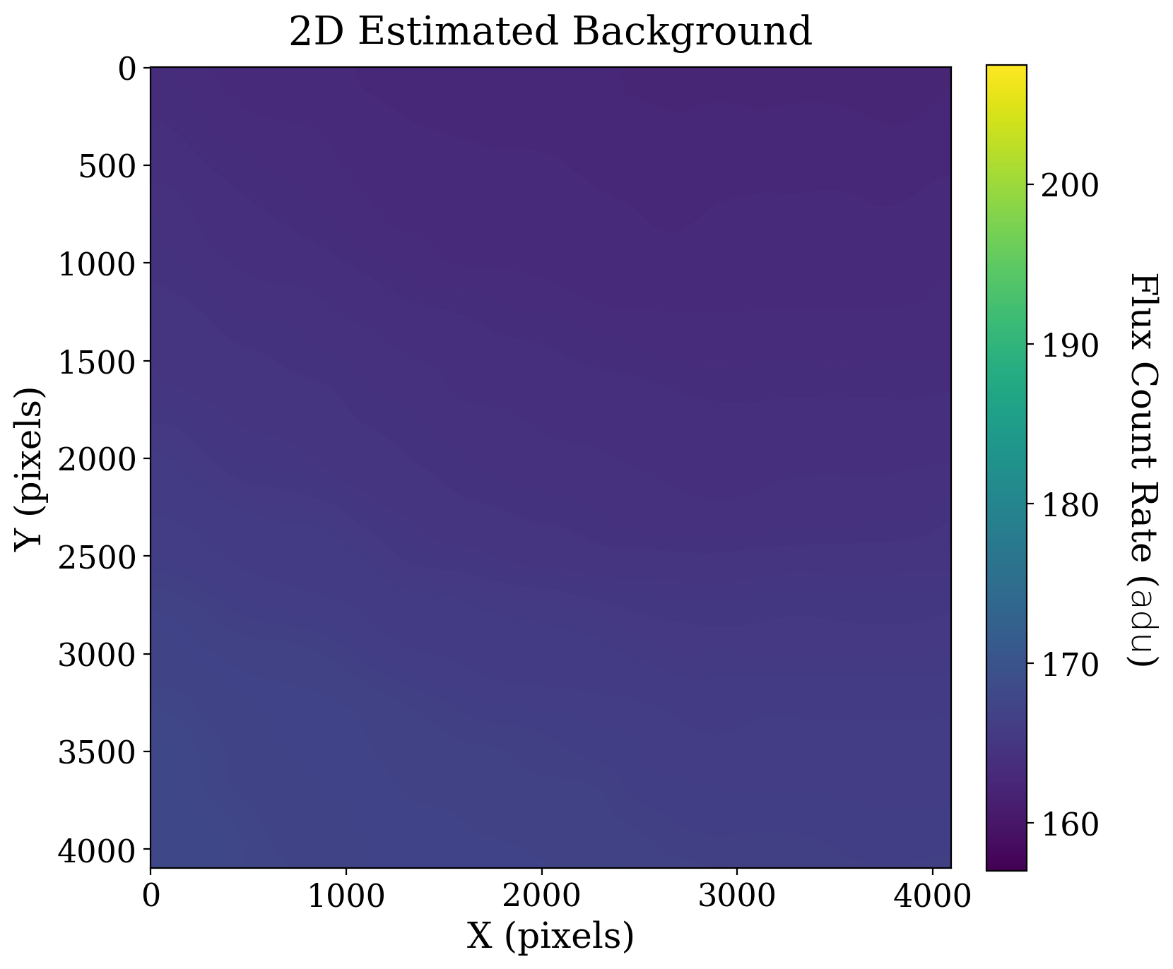
As expected, the gradient is clearly visible in the background. Next, we subtract that two-dimensional background and look at the result.

# Calculate the 2D background subtraction, maintaining metadata, unit, and mask
ccd_2d_bkgdsub = ccd_image.subtract(bkg.background)

# Set up the figure with subplots
fig, [ax1, ax2] = plt.subplots(1, 2, figsize=(12, 6), sharey=True)
plt.tight_layout()

fitsplot = ax1.imshow(ccd_scalar_bkgdsub, norm=norm_image_sub)

ax1.set_ylabel('Y (pixels)')
ax1.set_xlabel('X (pixels)')
ax1.set_title('Scalar Background-Subtracted Data')

# Plot the 2D-subtracted data
fitsplot = ax2.imshow(np.ma.masked_where(ccd_2d_bkgdsub.mask, ccd_2d_bkgdsub), norm=norm_image_sub)
ax2.set_xlabel('X (pixels)')
ax2.set_title('2D Background-Subtracted Data')

# Define the colorbar...
cbar_ax = fig.add_axes([1, 0.09, 0.03, 0.87])

cbar = fig.colorbar(fitsplot, cbar_ax)

cbar.set_label(r'Counts ({})'.format(ccd_image.unit.to_string('latex')),
               rotation=270, labelpad=30)

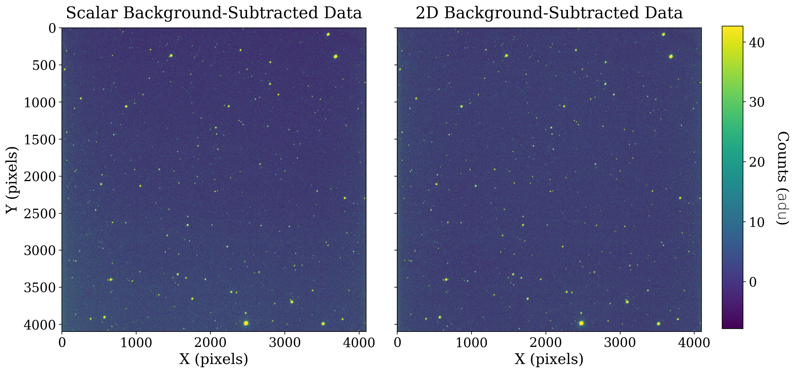
Note how much more even the 2D background-subtracted image looks; the difference between these two images is especially apparent in the bottom left and top right corners. This makes sense, as the background that Background2D identified was a gradient from the bottom left corner to the top right corner.