8.1.2. Handling masking before background removal

8.1.2.1. Data for this notebook

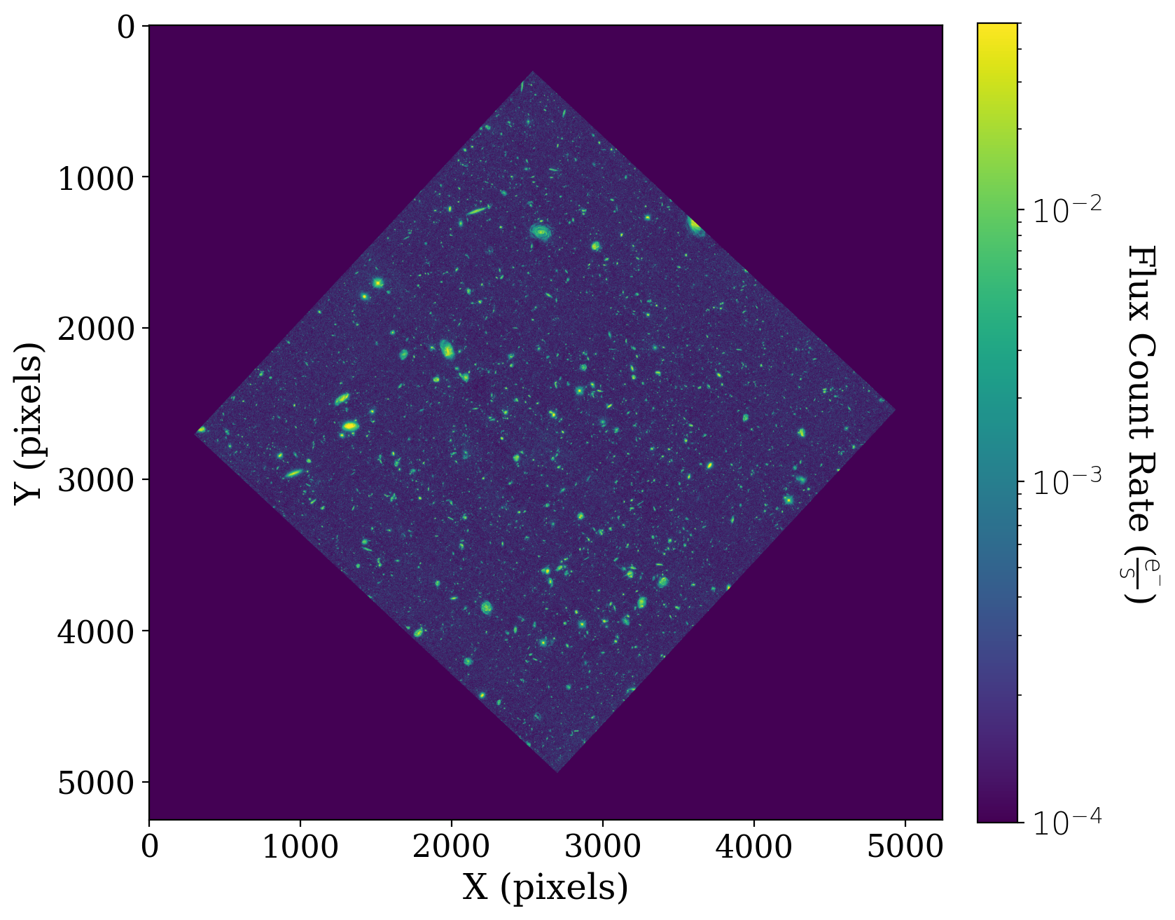
We will be manipulating Hubble eXtreme Deep Field (XDF) data, which was collected using the Advanced Camera for Surveys (ACS) on Hubble between 2002 and 2012. The image we use here is the result of 1.8 million seconds (500 hours!) of exposure time, and includes some of the faintest and most distant galaxies that had ever been observed.

Background subtraction is essential for accurate photometric analysis of astronomical data like the XDF.

The methods demonstrated here are also available in narrative from within the photutils.background documentation.

The original authors of this notebook were Lauren Chambers and Erik Tollerud.

8.1.2.2. Import necessary packages

First, let’s import packages that we will use to perform arithmetic functions and visualize data:

import numpy as np

from astropy.io import fits
from astropy.nddata import CCDData
import astropy.units as u
from astropy.stats import sigma_clipped_stats, SigmaClip
from astropy.visualization import ImageNormalize, LogStretch
import matplotlib.pyplot as plt
from matplotlib.ticker import LogLocator

from photutils.segmentation import detect_threshold, detect_sources
from photutils.utils import circular_footprint

# Show plots in the notebook
%matplotlib inline

Let’s also define some matplotlib parameters, such as title font size and the dpi, to make sure our plots look nice. To make it quick, we’ll do this by loading a style file shared with the other photutils tutorials into pyplot. We will use this style file for all the notebook tutorials. (See here to learn more about customizing matplotlib.)

plt.style.use('../photutils_notebook_style.mplstyle')

8.1.2.2.1. Data representation

Throughout this notebook, we are going to store our images in Python using a CCDData object (see Astropy documentation), which contains a numpy array in addition to metadata such as uncertainty, masks, or units. In this case, each image has units electrons (counts) per second.

Note that you could create the CCDData object directly from the URL where this image is taken from:

url = 'https://archive.stsci.edu/pub/hlsp/xdf hlsp_xdf_hst_acswfc-60mas_hudf_f435w_v1_sci.fits'
xdf_image = CCDData.read(url)

Since the data for the guide is meant to be downloaded in bulk before going through the guide, we read the image from disk here.

xdf_image = CCDData.read('hlsp_xdf_hst_acswfc-60mas_hudf_f435w_v1_sci.fits')

Let’s look at the data, including the background we’ve added. The cell below sets up an image normaliztaion we will use for all of our later views of the image. It also defines a small function, format_colorbar, that is used to set up the colorbar in the subsequent plots.

# Set up the figure with subplots
fig, ax1 = plt.subplots(1, 1, figsize=(8, 8))

# Set up the normalization and colormap. The values of vmin and vmax are specific to this image
norm_image = ImageNormalize(vmin=1e-4, vmax=5e-2, stretch=LogStretch())
cmap = plt.get_cmap('viridis')

# Plot the data, with pixels masked as appropriate
fitsplot = ax1.imshow(np.ma.masked_where(xdf_image.mask, xdf_image),
                      norm=norm_image, cmap=cmap)

# Define the colorbar
cbar = plt.colorbar(fitsplot, fraction=0.046, pad=0.04, ticks=LogLocator())

def format_colorbar(bar):
    # Add minor tickmarks
    bar.ax.yaxis.set_minor_locator(LogLocator(subs=range(1, 10)))

    # Force the labels to be displayed as powers of ten and only at exact powers of ten
    bar.ax.set_yticks([1e-4, 1e-3, 1e-2])
    labels = [f'$10^{{{pow:.0f}}}$' for pow in np.log10(bar.ax.get_yticks())]
    bar.ax.set_yticklabels(labels)

format_colorbar(cbar)

# Define labels
cbar.set_label(r'Flux Count Rate ({})'.format(xdf_image.unit.to_string('latex')),
               rotation=270, labelpad=30)
ax1.set_xlabel('X (pixels)')
ax1.set_ylabel('Y (pixels)');

8.1.2.3. Mask non-data portions of array

You probably noticed that a large portion of the data is equal to zero. The data we are using is a reduced mosaic that combines many different exposures, and that has been rotated such that not all of the array holds data.

We want to mask out the non-data portions of the image array, so all of those pixels that have a value of zero don’t interfere with our statistics and analyses of the data.

# Define the mask
xdf_image.mask = xdf_image.data == 0

# Set up the figure with subplots
fig, [ax1, ax2] = plt.subplots(1, 2, figsize=(12, 6), sharey=True)
plt.tight_layout()

# Plot the mask
ax1.imshow(xdf_image.mask, cmap='Greys')
ax1.set_xlabel('X (pixels)')
ax1.set_ylabel('Y (pixels)')
ax1.set_title('Mask')

# Plot the masked data
fitsplot = ax2.imshow(np.ma.masked_where(xdf_image.mask, xdf_image),
                      norm=norm_image, cmap=cmap)

# Define the colorbar and fix the labels
cbar_ax = fig.add_axes([1, 0.09, 0.03, 0.87])
cbar = fig.colorbar(fitsplot, cbar_ax, ticks=LogLocator())

format_colorbar(cbar)

cbar.set_label(r'Flux Count Rate ({})'.format(xdf_image.unit.to_string('latex')),
               rotation=270, labelpad=30)
ax2.set_xlabel('X (pixels)')
ax2.set_title('Masked Data');

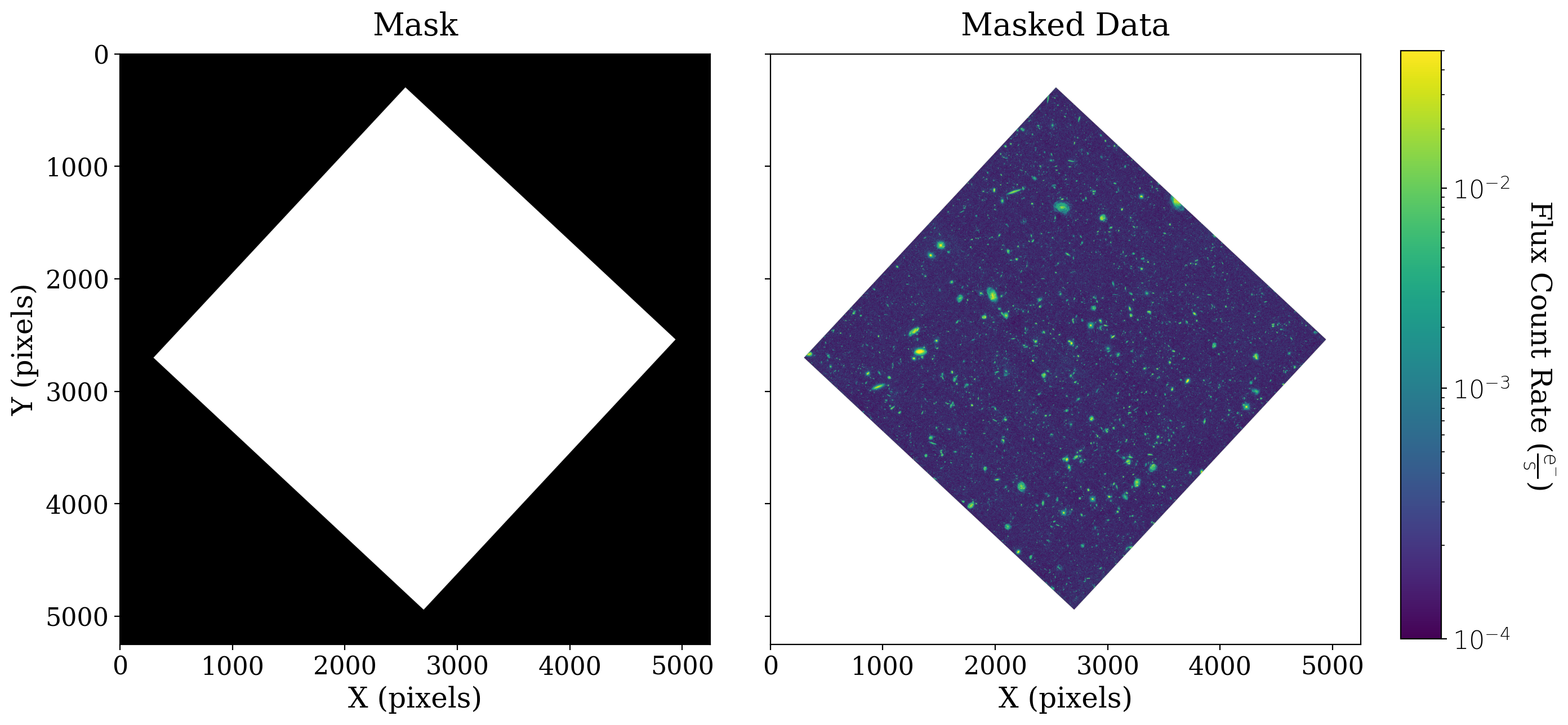
On the left we have plotted this mask, which has a value of 1 (or True) shown in black where the data is bad, and 0 (or False) shown in white where the data is good.

After the mask is applied to the data (on the right above) the data values “behind” the masked values are shown in white.

8.1.2.4. Perform scalar background estimation

Now that the data are properly masked, we can calculate some basic statistical values to do a scalar estimation of the image background.

Following the example in the previous section, we will estimate the background several ways.

By “scalar estimation”, we mean the calculation of a single value (such as the mean or median) to represent the value of the background for our entire two-dimensional dataset. This is in contrast to a two-dimensional background, where the estimated background is represented as an array of values that can vary spatially with the dataset. We will calculate a 2D background in the upcoming section.

8.1.2.4.1. Calculate scalar background value with sigma clipping

Here we will calculate the mean, median, and mode of the dataset using sigma clipping. With sigma clipping, the data is iteratively clipped to exclude data points outside of a certain sigma (standard deviation), thus removing some of the noise from the data before determining statistical values.

In the first case we account for the mask while sigma clipping and in the second case we do not.

# Calculate statistics with masking
mean, median, std = sigma_clipped_stats(xdf_image.data, sigma=3.0, maxiters=5, mask=xdf_image.mask)

# Calculate statistics without masking
stats_nomask = sigma_clipped_stats(xdf_image.data, sigma=3.0, maxiters=5)

8.1.2.4.2. Calculate scalar background value without sigma clipping

Here we will calculate the mean, median, and mode of the dataset without using sigma clipping.

As above, we do this first taking into account the mask and then ignoring the mask.

mean_noclip_mask = np.mean(xdf_image.data[~xdf_image.mask])
median_noclip_mask = np.median(xdf_image.data[~xdf_image.mask])

mean_noclip_nomask = np.mean(xdf_image.data)
median_noclip_nomask = np.median(xdf_image.data)

8.1.2.4.3. Mask sources, then calculate scalar background

As discussed in the section on background estimation with a simulated image, the most accurate estimate of the scalar background is obtained when the sources are masked first. The cell below does that procedure.

# Set up sigma clipping
sigma_clip = SigmaClip(sigma=3.0, maxiters=10)

threshold = detect_threshold(xdf_image.data, nsigma=2.0, sigma_clip=sigma_clip, mask=xdf_image.mask)
segment_img = detect_sources(xdf_image.data, threshold, npixels=10, mask=xdf_image.mask)
footprint = circular_footprint(radius=10)

# Make the source mask a circle of radius 10 around each detected source
source_mask = segment_img.make_source_mask(footprint=footprint)

# Combine the source mask with the data mask
full_mask = source_mask | xdf_image.mask

# Compute the stats
source_mask_clip_mean, source_mask_clip_med, source_mask_clip_std  = sigma_clipped_stats(xdf_image.data, sigma=3, mask=full_mask)

8.1.2.4.4. Compare the background estimates

But what difference does this sigma clipping make? And how important is masking, anyway? Let’s visualize these statistics to get an idea:

# Set up the figure with subplots
fig, [ax1, ax2] = plt.subplots(1, 2, figsize=(12, 4), sharey=True)

# Plot histograms of the data
flux_range = (-.5e-3, 1.5e-3)
ax1.hist(xdf_image.data[~xdf_image.mask], bins=100, range=flux_range)
ax2.hist(xdf_image.data[~xdf_image.mask], bins=100, range=flux_range)

# Plot lines for each kind of mean
ax1.axvline(mean, label='Non-data masked and Clipped', c='C1', ls='-.', lw=3)
ax1.axvline(mean_noclip_mask, label='Masked', c='C2', lw=3)
ax1.axvline(stats_nomask[0], label='Clipped', c='C3', ls=':', lw=5)
ax1.axvline(source_mask_clip_mean, label='Sources masked and clipped', c='C4', lw=3)
ax1.axvline(mean_noclip_nomask, label='Neither', c='C5', ls='--', lw=3)

ax1.set_xlim(flux_range)
ax1.set_xlabel(r'Flux Count Rate ({})'.format(xdf_image.unit.to_string('latex')), fontsize=14)
ax1.set_ylabel('Frequency', fontsize=14)
ax1.set_title('Effect of Sigma-Clipping \n and Masking on Mean', fontsize=16)

# Plot lines for each kind of median
# Note: use np.ma.median rather than np.median for masked arrays
ax2.axvline(median, label='Non-data masked and Clipped', c='C1', ls='-.', lw=3)
ax2.axvline(median_noclip_mask, label='Masked', c='C2', lw=3)
ax2.axvline(source_mask_clip_med, label='Sources masked and clipped', c='C4', lw=3)
ax2.axvline(stats_nomask[1], label='Clipped', c='C3', ls=':', lw=5)
ax2.axvline(median_noclip_nomask, label='Neither', c='C5', ls='--', lw=3)


ax2.set_xlim(flux_range)
ax2.set_xlabel(r'Flux Count Rate ({})'.format(xdf_image.unit.to_string('latex')), fontsize=14)
ax2.set_title('Effect of Sigma-Clipping \n and Masking on Median', fontsize=16)

# Add legend
ax1.legend(fontsize=11, loc='lower center', bbox_to_anchor=(1.1, -0.55), ncol=2, handlelength=6);

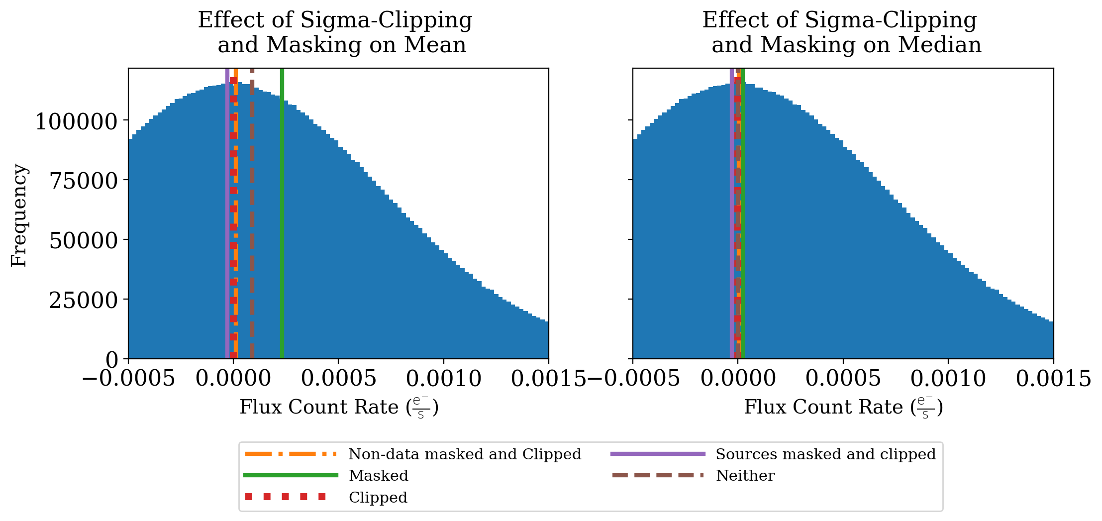
Masking makes a big difference to the mean in this case because so many of the pixels in the original image contain no data. Sigma clipping also makes some difference, moving the mean value closer to zero. Masking out the sources moves the mean below zero, which is not surprising in this case. The distribution of pixels is clearly near zero, and masking out the sources means removing the largest positive values.

Note that the median is about the same no matter which approach you use.

8.1.2.4.5. Subtract scalar background value

But enough looking at numbers, let’s actually remove the background from the data. By using the subtract() method of the CCDData class, we can subtract the mean background while maintaining the metadata and mask of our original CCDData object:

# Calculate the scalar background subtraction, maintaining metadata, unit, and mask
xdf_scalar_bkgdsub = xdf_image.subtract(mean * u.electron / u.s)

# Set up the figure with subplots
fig, [ax1, ax2] = plt.subplots(1, 2, figsize=(12, 6), sharey=True)
plt.tight_layout()

# Plot the original data
fitsplot = ax1.imshow(np.ma.masked_where(xdf_image.mask, xdf_image), norm=norm_image)
ax1.set_xlabel('X (pixels)')
ax1.set_ylabel('Y (pixels)')
ax1.set_title('Original Data')

# Plot the subtracted data
fitsplot = ax2.imshow(np.ma.masked_where(xdf_scalar_bkgdsub.mask, xdf_scalar_bkgdsub), norm=norm_image)
ax2.set_xlabel('X (pixels)')
ax2.set_title('Scalar Background-Subtracted Data')

# Define the colorbar...
cbar_ax = fig.add_axes([1, 0.09, 0.03, 0.87])

cbar = fig.colorbar(fitsplot, cbar_ax, ticks=LogLocator())

format_colorbar(cbar)

cbar.set_label(r'Flux Count Rate ({})'.format(xdf_image.unit.to_string('latex')),
               rotation=270, labelpad=30)

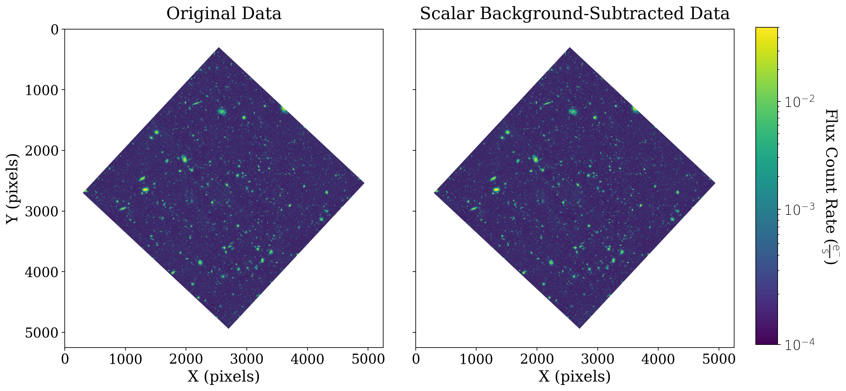
Note that both plots above use the same normalization scheme, represented by the colorbar on the right. That is to say, if two pixels have the same color in both arrays, they have the same value.

Subtracting the scalar background does not have much effect here because the background is so close to zero.

One note about keeping the color scale the same, as we do in this example: if there is a significant scalar background then the effect of scalar background subtraction will be to simply make the entire image look darker. That will be illustrated in the example in the next section of the guide.

8.1.2.5. Perform 2-D background estimation

The Background2D class in photutils allows users to model 2-dimensional backgrounds, by calculating the mean or median in small boxes, and smoothing these boxes to reconstruct a continuous 2D background. The class includes the following arguments/attributes:

• box_size — the size of the boxes used to calculate the background. This should be larger than individual sources, yet still small enough to encompass changes in the background.

• filter_size — the size of the median filter used to smooth the final 2D background. The dimension should be odd along both axes.

• filter_threshold — threshold below which the smoothing median filter will not be applied.

• sigma_clip — an astropy.stats.SigmaClip object that is used to specify the sigma and number of iterations used to sigma-clip the data before background calculations are performed.

• bkg_estimator — the method used to perform the background calculation in each box (mean, median, SExtractor algorithm, etc.).

For this example, we will use the MeanBackground estimator. Note though, that there is little or no spatial variation apparent in the background of this image.

from photutils.background import Background2D, MeanBackground

sigma_clip = SigmaClip(sigma=3., maxiters=5)
bkg_estimator = MeanBackground()
bkg = Background2D(xdf_image, box_size=200, filter_size=(9, 9), mask=xdf_image.mask,
                   sigma_clip=sigma_clip, bkg_estimator=bkg_estimator)

So, what does this 2D background look like? Where were the boxes placed?

# Set up the figure with subplots
fig, ax1 = plt.subplots(1, 1, figsize=(8, 8))

# Plot the background
fitsplot = ax1.imshow(np.ma.masked_where(xdf_image.mask, bkg.background.data ), norm=norm_image)

# Plot the meshes
bkg.plot_meshes(outlines=True, color='lightgrey')

# Define the colorbar
cbar = plt.colorbar(fitsplot, fraction=0.046, pad=0.04, ticks=LogLocator())

format_colorbar(cbar)

# Define labels
cbar.set_label(r'Flux Count Rate ({})'.format(xdf_image.unit.to_string('latex')),
               rotation=270, labelpad=30)
ax1.set_xlabel('X (pixels)')
ax1.set_ylabel('Y (pixels)')
ax1.set_title('2D Estimated Background');

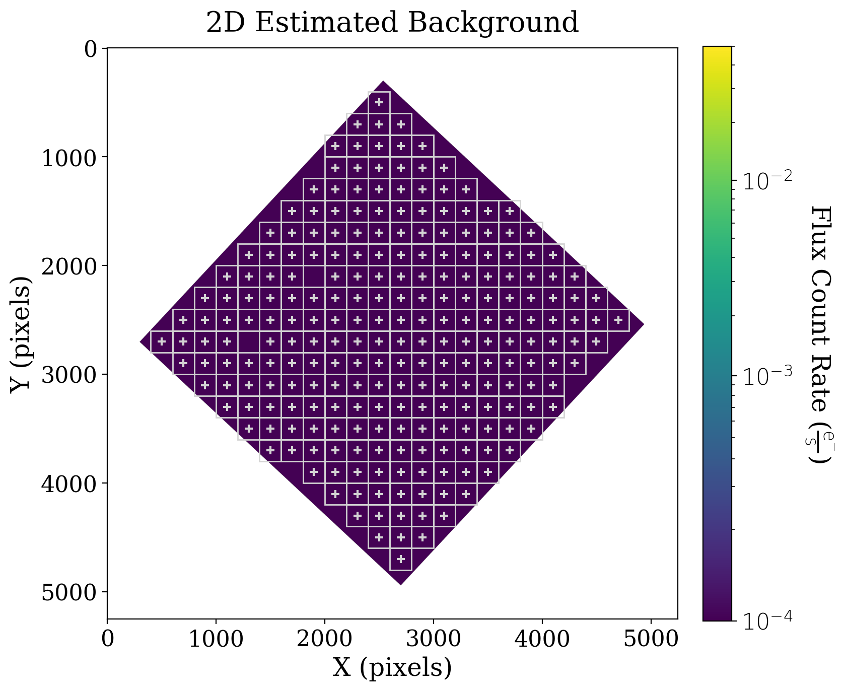
You might notice that not all areas of the background array have mesh boxes over them (look for those boxes that do not have a +). If you compare this background array with the original data, you’ll see that these un-boxed areas contain particularly bright sources, and thus are not being included in the background estimate.

The background is also, as we expected in this case, close to uniform.

And how does the data look if we use this background subtraction method (again maintaining the attributes of the CCDData object)?

# Calculate the 2D background subtraction, maintaining metadata, unit, and mask
xdf_2d_bkgdsub = xdf_image.subtract(bkg.background)

# Set up the figure with subplots
fig, [ax1, ax2] = plt.subplots(1, 2, figsize=(12, 6), sharey=True)
plt.tight_layout()

# Plot the scalar-subtracted data
fitsplot = ax1.imshow(np.ma.masked_where(xdf_scalar_bkgdsub.mask, xdf_scalar_bkgdsub), norm=norm_image)
cbar.set_label(r'Flux Count Rate ({})'.format(xdf_image.unit.to_string('latex')),
               rotation=270, labelpad=30)
ax1.set_ylabel('Y (pixels)')
ax1.set_xlabel('X (pixels)')
ax1.set_title('Scalar Background-Subtracted Data')

# Plot the 2D-subtracted data
fitsplot = ax2.imshow(np.ma.masked_where(xdf_2d_bkgdsub.mask, xdf_2d_bkgdsub), norm=norm_image)
ax2.set_xlabel('X (pixels)')
ax2.set_title('2D Background-Subtracted Data')

# Define the colorbar...
cbar_ax = fig.add_axes([1, 0.09, 0.03, 0.87])

cbar = fig.colorbar(fitsplot, cbar_ax, ticks=LogLocator())
cbar.ax.yaxis.set_minor_locator(LogLocator(subs=range(1, 10)))

# ...and force the labels to be displayed as powers of ten
cbar.ax.set_yticks([1e-4, 1e-3, 1e-2])
labels = [f'$10^{{{pow:.0f}}}$' for pow in np.log10(cbar.ax.get_yticks())]
cbar.ax.set_yticklabels(labels)

cbar.set_label(r'Flux Count Rate ({})'.format(xdf_image.unit.to_string('latex')),
               rotation=270, labelpad=30)

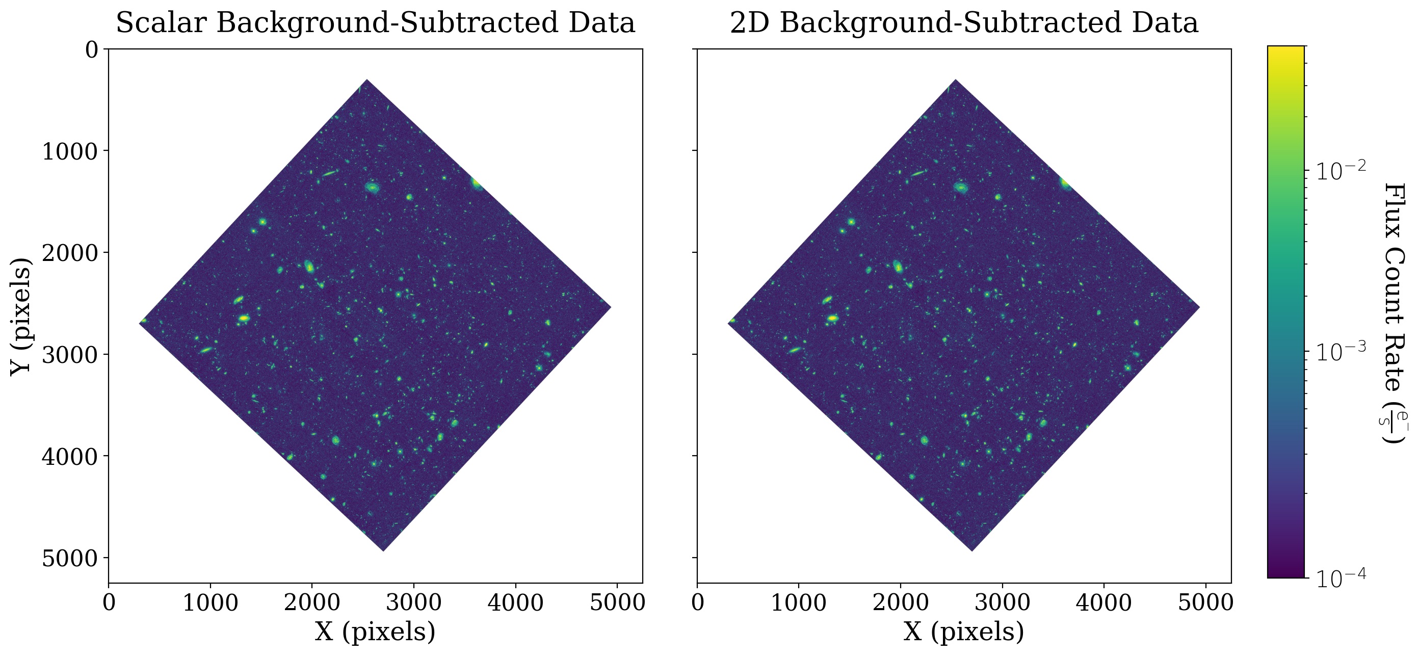
In this case 2D background subtraction was not necessary, as you might expect from an image like the XDF that has already been processed.

In the next section we look at an image that does have a gradient in the background from moonlight.