8.3.1. Peak finding#
8.3.1.1. Simulated image of galaxies and stars#
In the first part of this notebook we consider an image that includes 100 sources, all with Gaussian profiles, some of which are fairly elongated. We used this image in the previous section about removing the background prior to source detection.
As usual, we begin with some imports.
import warnings

from astropy.stats import sigma_clipped_stats
from astropy.visualization import SqrtStretch
from astropy.visualization.mpl_normalize import ImageNormalize

import matplotlib.pyplot as plt

from photutils.centroids import centroid_2dg
from photutils.datasets import make_100gaussians_image
from photutils.detection import find_peaks, DAOStarFinder

plt.style.use('../photutils_notebook_style.mplstyle')
/usr/share/miniconda/envs/test/lib/python3.11/site-packages/tqdm/auto.py:21: TqdmWarning: IProgress not found. Please update jupyter and ipywidgets. See https://ipywidgets.readthedocs.io/en/stable/user_install.html
  from .autonotebook import tqdm as notebook_tqdm
To begin, let’s create the image and subtract the background. Recall that this image contains a mix of star-like object and more extended sources.
data = make_100gaussians_image()
mean, med, std = sigma_clipped_stats(data, sigma=3.0, maxiters=5)
data_subtracted = data - med
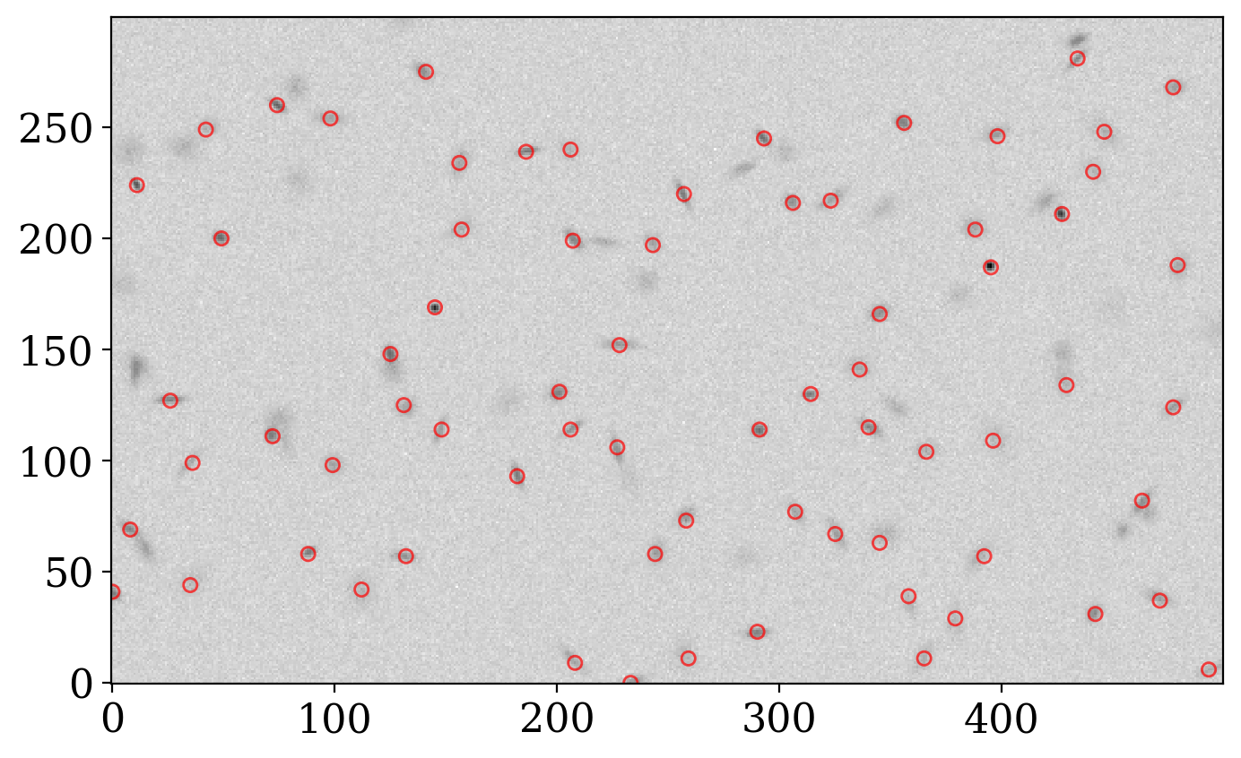
8.3.1.2. Source Detection with peak finding#
For more general source detection cases that do not require comparison with models, photutils offers the find_peaks function.
This function simply finds sources by identifying local maxima above a given threshold and separated by a given distance, rather than trying to fit data to a given model. Unlike the previous detection algorithms, find_peaks does not necessarily calculate objects’ centroids. Unless the centroid_func argument is passed a function like photutils.centroids.centroid_2dg that can handle source position centroiding, find_peaks will return just the integer value of the peak pixel for each source.
This algorithm is particularly useful for identifying non-stellar sources or heavily distorted sources in image data.
The centroid-finding, which we do here only so that we can compare positions found by this method to positions found by the star-finding methods, can generate many warnings when an attempt is made to fit a 2D Gaussian to the sources. The warnings are suppressed below to avoid cluttering the output.
Let’s see how it does:
with warnings.catch_warnings(action="ignore"):
    sources_findpeaks = find_peaks(data_subtracted,
                                   threshold=5. * std, box_size=29,
                                   centroid_func=centroid_2dg)
print(sources_findpeaks)
 id x_peak y_peak     peak_value         x_centroid         y_centroid
--- ------ ------ ------------------ ------------------ ------------------
  1    233      0 22.633606464239687 234.30738293708558 0.3252266052191978
  2    493      6 13.546963965223004 494.12995930395266  5.943363133749774
  3    208      9 17.346874844390104  207.1353444191415 10.355528979836118
  4    259     11 11.248467564978402  257.8424994073731  12.22974776870233
  5    365     11 12.637249593274138   364.867390818497 11.150125973145085
  6    290     23  28.98909001390059 289.81151483546637 22.313288287707437
  7    379     29 10.906120071732058  379.2803321166154 27.853170351023564
  8    442     31 27.009595861523184  441.3447657982843   31.2025570678272
  9    471     37 18.989486145201486 470.66144861033956  38.17650929613494
 10    358     39 13.519122776424464 358.56678372121416 36.006729560780045
...    ...    ...                ...                ...                ...
 62    293    245  38.69510036786478  292.6447379137065 245.03659043033807
 63    398    246 18.775975076986878  397.3006114275939 246.99272806526454
 64    446    248 13.906635070560856  446.7634329138691 247.68128784414358
 65     42    249 13.256323329550764 35.098308269088044 243.29612818684046
 66    356    252  30.00969198273592  355.5325295364271  252.1937672284385
 67     98    254 15.847143478097742  97.92272437224054 254.08791107756423
 68     74    260  47.35429493883031  74.39131328124375 259.77579784397756
 69    477    268 17.870494505057362  477.9120830493799  267.9335268954686
 70    141    275 23.127844438211586 139.71393211621677  275.1800460996928
 71    434    281 28.311057338166965 434.12851029483994  286.1724452349321
Length = 71 rows
# Set up the figure with subplots
fig, ax1 = plt.subplots(1, 1, figsize=(8, 8))

norm = ImageNormalize(stretch=SqrtStretch())
fitsplot = ax1.imshow(data, cmap='Greys', origin='lower', norm=norm,
           interpolation='nearest')
ax1.scatter(sources_findpeaks['x_peak'], sources_findpeaks['y_peak'], s=30, marker='o',
            lw=1, alpha=0.7, facecolor='None', edgecolor='r');
8.3.1.3. Comparing Detection Methods#
Let’s compare how peak finding compares to using DAOStarFinder on this image.
detect_fwhm = 5.0
daofind = DAOStarFinder(fwhm=detect_fwhm, threshold=5.*std)
sources_dao = daofind(data_subtracted)
print(f'''DAOStarFinder: {len(sources_dao)} sources
find_peaks: {len(sources_findpeaks)} sources''')
DAOStarFinder: 48 sources
find_peaks: 71 sources
Let’s plot both sets of sources on the original image.
fig, ax1 = plt.subplots(1, 1, figsize=(8, 8))

# Plot the data
fitsplot = ax1.imshow(data, norm=norm, cmap='Greys', origin='lower')

marker_size = 60
ax1.scatter(sources_findpeaks['x_peak'], sources_findpeaks['y_peak'], s=marker_size, marker='s',
            lw=1, alpha=1, facecolor='None', edgecolor='r', label='Found by find_peaks')
ax1.scatter(sources_dao['xcentroid'], sources_dao['ycentroid'], s=2 * marker_size, marker='D',
            lw=1, alpha=1, facecolor='None', edgecolor='#0077BB', label='Found by DAOfind')

# Add legend
ax1.legend(ncol=2, loc='lower center', bbox_to_anchor=(0.5, -0.35))


ax1.set_xlabel('X (pixels)')
ax1.set_ylabel('Y (pixels)')
ax1.set_title('Sources Found by Different Methods');
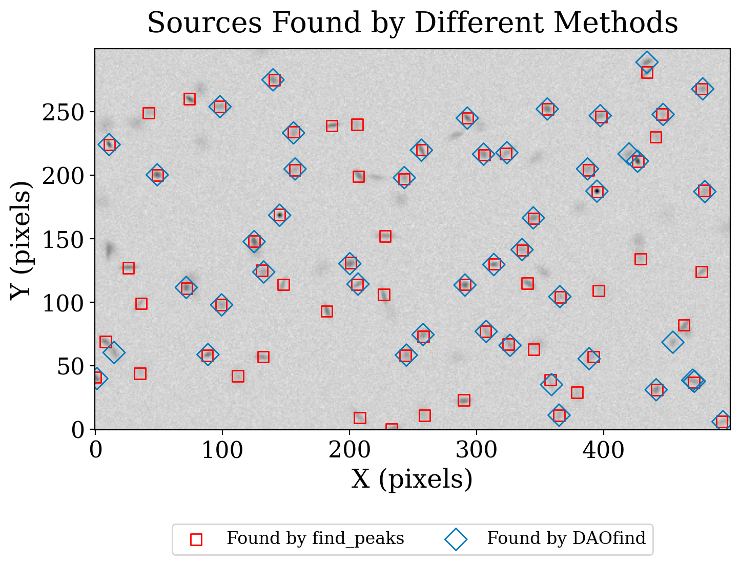
That peak findging works better on this image that DAOfind shouldn’t be surprising because many of the sources are not round. As we discussed in the section on source detection in a simulated image, the star-finding techniques are not a good match for an image like this with many extended sources.
8.3.1.4. Summary#
There are several more sources found by find_peaks than are found found by the star-finding algorithms, but several are still being missed. In the section on image segmentation with a simulated image we will look at a much different approach that is especially well suited to finding extended objects.