8.3.2. Peak finding in the XDF

8.3.2.1. Data for this notebook

We will be manipulating Hubble eXtreme Deep Field (XDF) data, which was collected using the Advanced Camera for Surveys (ACS) on Hubble between 2002 and 2012. The image we use here is the result of 1.8 million seconds (500 hours!) of exposure time, and includes some of the faintest and most distant galaxies that had ever been observed.

The methods demonstrated here are also available in the photutils.detection documentation.

The original authors of this notebook were Lauren Chambers, Erik Tollerud and Tom Wilson.

We begin with imports.

import warnings

from astropy.nddata import CCDData
from astropy.stats import sigma_clipped_stats, SigmaClip
import astropy.units as u
from astropy.visualization import ImageNormalize, LogStretch

import matplotlib.pyplot as plt
from matplotlib.ticker import LogLocator

import numpy as np

from photutils.background import Background2D, MeanBackground
from photutils.centroids import centroid_2dg
from photutils.detection import find_peaks, DAOStarFinder, IRAFStarFinder

# Show plots in the notebook
%matplotlib inline

Next, we load the image and calculate the background statistics.

xdf_image = CCDData.read('hlsp_xdf_hst_acswfc-60mas_hudf_f435w_v1_sci.fits')
# Define the mask
mask = xdf_image.data == 0
xdf_image.mask = mask

mean, median, std = sigma_clipped_stats(xdf_image.data, sigma=3.0, maxiters=5, mask=xdf_image.mask)

plt.style.use('../photutils_notebook_style.mplstyle')

8.3.2.2. Source Detection with peak finding

For more general source detection cases that do not require comparison with models, photutils offers the find_peaks function.

This function simply finds sources by identifying local maxima above a given threshold and separated by a given distance, rather than trying to fit data to a given model. Unlike the previous detection algorithms, find_peaks does not necessarily calculate objects’ centroids. Unless the centroid_func argument is passed a function like photutils.centroids.centroid_2dg that can handle source position centroiding, find_peaks will return just the integer value of the peak pixel for each source.

The centroid-finding, which we do here only so that we can compare positions found by this method to positions found by the star-finding methods, can generate many warnings when an attempt is made to fit a 2D Gaussian to the sources. The warnings are suppressed below to avoid cluttering the output.

Let’s see how it does:

with warnings.catch_warnings(action="ignore"):
    sources_findpeaks = find_peaks(xdf_image.data - median, mask=xdf_image.mask,
                                   threshold=20. * std, box_size=29,
                                   centroid_func=centroid_2dg)
print(sources_findpeaks)

 id  x_peak y_peak  peak_value     x_centroid         y_centroid    
---- ------ ------ ----------- ------------------ ------------------
   1   2525    393  0.13548362 2525.7825499490064 393.88055503239474
   2   2466    400 0.029366337 2465.7798479347243 398.05573502870715
   3   2552    459 0.018309232  2553.144113059114  458.5071866239441
   4   2614    463 0.018226365 2612.9628856780873 463.90212782823716
   5   2635    471 0.021132588 2635.6120154601685 473.07924452934066
   6   2635    493  0.08027035 2634.6718726918175  492.2803943395769
   7   2678    496 0.026410304 2677.4804921300647  496.9715217867422
   8   2586    507 0.037171733  2585.462527787139  507.3101665735999
   9   2326    554 0.018130405  2325.528858931348  553.6418835727972
  10   2616    560 0.021488318  2615.938885064026  559.9740345848103
 ...    ...    ...         ...                ...                ...
1024   2836   4662  0.01867783  2828.840372102822  4661.979368247575
1025   2956   4663 0.030241651   2957.43798265238  4664.380775142155
1026   2814   4664 0.016782979  2818.781489666815  4662.160254025871
1027   2452   4711  0.04217213 2449.2187375121634  4711.273878402247
1028   2631   4712 0.015904581  2630.494634031711  4712.276375599891
1029   2676   4733 0.014843852 2676.3994552743634  4733.100046176483
1030   2549   4736 0.015206217 2551.5624408418103  4733.959834146592
1031   2878   4736  0.03463787 2879.7315243346816  4737.664616308867
1032   2607   4758 0.019089993  2603.851675357389   4761.25199341925
1033   2515   4764  0.02098297 2499.6013132419002  4716.863606119463
Length = 1033 rows

There are roughly 1,000 sources identified in the image. Recall from the notebook on star-finding detection methods that roughly 1,500 sources were found with DAOStarFinder.

# Set up the figure with subplots
fig, ax1 = plt.subplots(1, 1, figsize=(8, 8))

# Plot the data
# Set up the normalization and colormap
norm_image = ImageNormalize(vmin=1e-4, vmax=5e-2, stretch=LogStretch(), clip=False)
cmap = plt.get_cmap('viridis')
cmap.set_bad('white') # Show masked data as white
fitsplot = ax1.imshow(np.ma.masked_where(xdf_image.mask, xdf_image.data),
                      norm=norm_image, cmap=cmap)
ax1.scatter(sources_findpeaks['x_peak'], sources_findpeaks['y_peak'], s=30, marker='o',
            lw=1, alpha=0.7, facecolor='None', edgecolor='r')

# Define the colorbar
cbar = plt.colorbar(fitsplot, fraction=0.046, pad=0.04, ticks=LogLocator())

def format_colorbar(bar):
    # Add minor tickmarks
    bar.ax.yaxis.set_minor_locator(LogLocator(subs=range(1, 10)))

    # Force the labels to be displayed as powers of ten and only at exact powers of ten
    bar.ax.set_yticks([1e-4, 1e-3, 1e-2])
    labels = [f'$10^{{{pow:.0f}}}$' for pow in np.log10(bar.ax.get_yticks())]
    bar.ax.set_yticklabels(labels)

format_colorbar(cbar)

# Define labels
cbar.set_label(r'Flux Count Rate ({})'.format(xdf_image.unit.to_string('latex')),
               rotation=270, labelpad=30)
ax1.set_xlabel('X (pixels)')
ax1.set_ylabel('Y (pixels)')
ax1.set_title('find_peaks Sources');

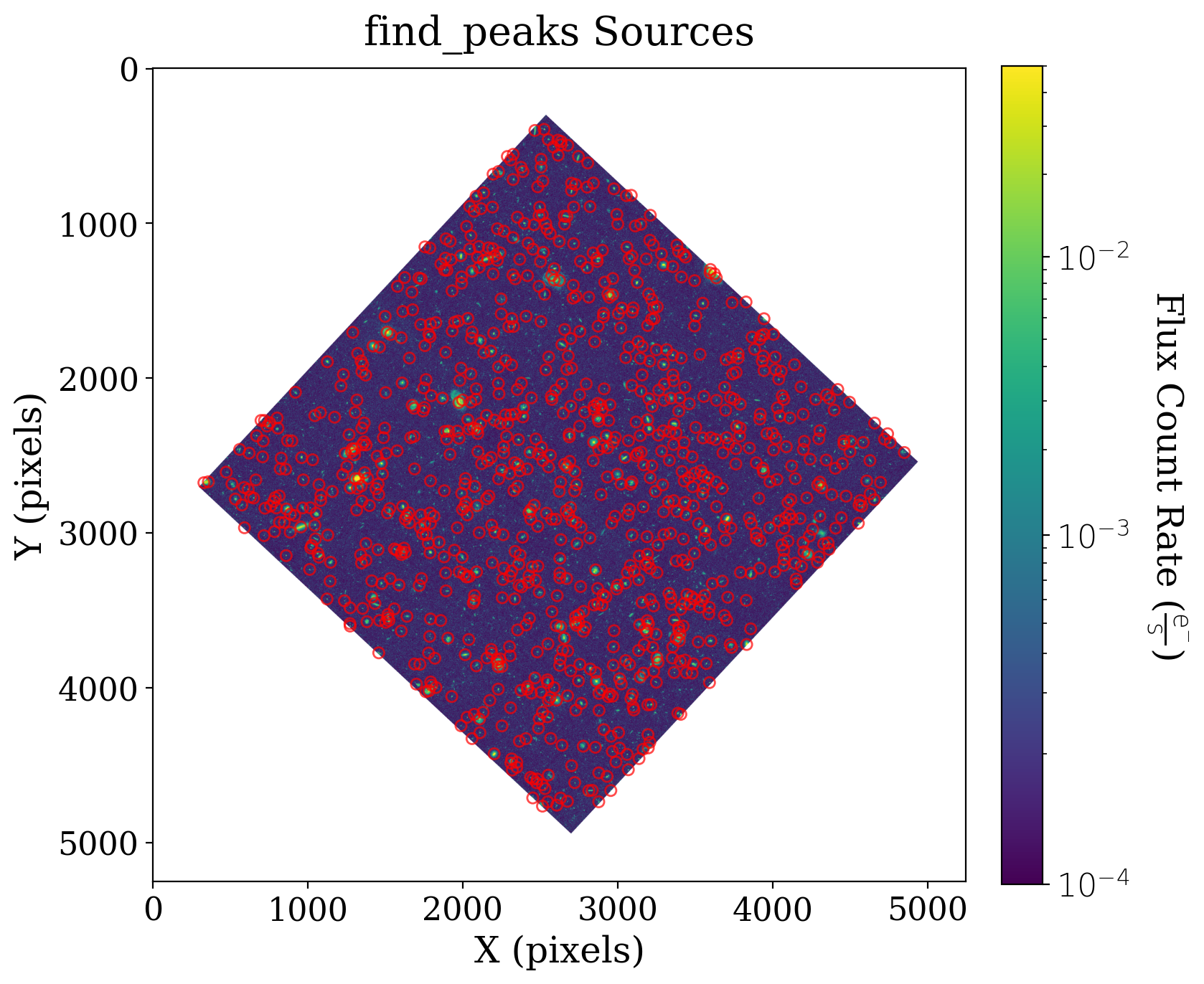
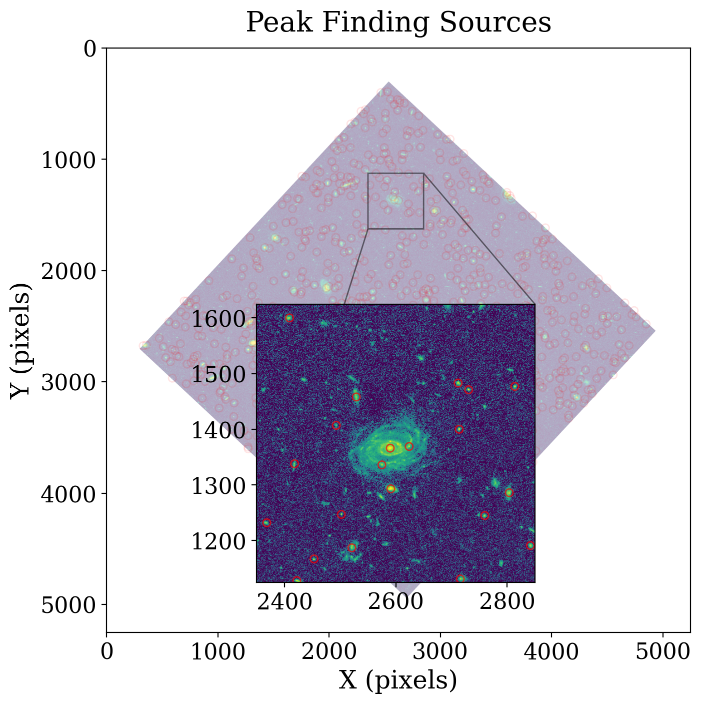
We once again look at region around the large galaxy. A comparison of this approach with the star-finding approaches appears later in this section.

fig, ax = plt.subplots(figsize=(8, 8))
top = 1125
left = 2350
cutout_size = 500
inset_display_size = 5 * cutout_size

fitsplot = ax.imshow(xdf_image, cmap=cmap, norm=norm_image, alpha=0.4)
ax.scatter(sources_findpeaks['x_peak'], sources_findpeaks['y_peak'], s=30, marker='o',
           lw=1, alpha=0.1, facecolor='None', edgecolor='r')

ax.set_xlabel('X (pixels)')
ax.set_ylabel('Y (pixels)')
ax.set_title('Peak Finding Sources')

ax2 = ax.inset_axes([2600 - inset_display_size // 2, 2300, inset_display_size, inset_display_size], 
                    xlim=(left, left + cutout_size), ylim=(top, top + cutout_size),
                    transform=ax.transData)
ax.indicate_inset_zoom(ax2, edgecolor="black")

ax2.imshow(xdf_image, cmap=cmap, norm=norm_image)

in_region = (
    (left < sources_findpeaks['x_peak']) &
    (sources_findpeaks['x_peak'] < (left + cutout_size)) & 
    (top < sources_findpeaks['y_peak']) &
    (sources_findpeaks['y_peak'] < (top + cutout_size))
)
sources_findpeaks_to_plot = sources_findpeaks[in_region]
ax2.scatter(sources_findpeaks_to_plot['x_peak'], sources_findpeaks_to_plot['y_peak'], s=30, marker='o',
            lw=1, alpha=0.7, facecolor='None', edgecolor='r');

8.3.2.3. Comparing Detection Methods

Let’s compare how each of these different strategies did.

First, we repeat our earlier detection using DAOStarFinder and IRAFStarFinder.

daofind = DAOStarFinder(fwhm=5.0, threshold=20. * std)
sources_dao = daofind(np.ma.masked_where(xdf_image.mask, xdf_image))

iraffind_match = IRAFStarFinder(fwhm=5.0, threshold=20. * std,
                                sharplo=0.2, sharphi=1.0,
                                roundlo=-1.0, roundhi=1.0,
                                minsep_fwhm=0.0)
sources_iraf_match = iraffind_match(np.ma.masked_where(xdf_image.mask, xdf_image))

print(f'''DAOStarFinder: {len(sources_dao)} sources
IRAFStarFinder: {len(sources_iraf_match)} sources
find_peaks: {len(sources_findpeaks)} sources''') 

DAOStarFinder: 1470 sources
IRAFStarFinder: 1415 sources
find_peaks: 1033 sources

Next, how many of these sources match? We can answer this question by using sets to compare the centroids of the different sources (rounding to the nearest integer).

# Make lists of centroid coordinates
centroids_dao = [(x, y) for x, y in sources_dao['xcentroid', 'ycentroid']]
centroids_iraf = [(x, y) for x, y in sources_iraf_match['xcentroid', 'ycentroid']]
centroids_findpeaks = [(x, y) for x, y in sources_findpeaks['x_centroid', 'y_centroid']]

# Round those coordinates to the ones place and convert them to be sets
rounded_centroids_dao = set([(round(x, 0), round(y, 0)) for x, y in centroids_dao])
rounded_centroids_iraf = set([(round(x, 0), round(y, 0)) for x, y in centroids_iraf])
rounded_centroids_findpeaks = set([(round(x, 0), round(y, 0)) for x, y in centroids_findpeaks])

# Examine the intersections of different sets to determine which sources are shared
all_match = rounded_centroids_dao.intersection(rounded_centroids_iraf).intersection(rounded_centroids_findpeaks)
dao_iraf_match = rounded_centroids_dao.intersection(rounded_centroids_iraf)
dao_findpeaks_match = rounded_centroids_dao.intersection(rounded_centroids_findpeaks)
iraf_findpeaks_match = rounded_centroids_iraf.intersection(rounded_centroids_findpeaks)

print(f'''Matching sources found by:
    All methods: {len(all_match)}
    DAOStarFinder & IRAFStarFinder: {len(dao_iraf_match)}
    DAOStarFinder & find_peaks: {len(dao_findpeaks_match)}
    IRAFStarFinder & find_peaks: {len(iraf_findpeaks_match)}''')

Matching sources found by:
    All methods: 172
    DAOStarFinder & IRAFStarFinder: 975
    DAOStarFinder & find_peaks: 191
    IRAFStarFinder & find_peaks: 213

And just for fun, let’s plot these matching sources. (The colors chosen to represent different sets are from Paul Tol’s guide for accessible color schemes.)

# Set up the figure with subplots
fig, ax1 = plt.subplots(1, 1, figsize=(8, 8))

# Plot the data
fitsplot = ax1.imshow(np.ma.masked_where(xdf_image.mask, xdf_image), norm=norm_image)
ax1.scatter([x for x, y in list(dao_findpeaks_match)], [y for x, y in list(dao_findpeaks_match)],
            s=30, marker='s', lw=1,  facecolor='None', edgecolor='#EE7733',
            label='Found by DAO and find_peaks')
ax1.scatter([x for x, y in list(dao_iraf_match)], [y for x, y in list(dao_iraf_match)],
            s=30, marker='D', lw=1, facecolor='None', edgecolor='#EE3377',
            label='Found by DAO and IRAF')
ax1.scatter([x for x, y in list(iraf_findpeaks_match)], [y for x, y in list(iraf_findpeaks_match)],
            s=30, marker='o', lw=1, facecolor='None', edgecolor='#0077BB',
            label='Found by IRAF and find_peaks')
ax1.scatter([x for x, y in list(all_match)], [y for x, y in list(all_match)],
            s=30, marker='o', lw=1.2, linestyle=':',facecolor='None', edgecolor='#BBBBBB',
            label='Found by all methods')

# Add legend
ax1.legend(ncol=2, loc='lower center', bbox_to_anchor=(0.5, -0.25))

# Define labels
ax1.set_xlabel('X (pixels)')
ax1.set_ylabel('Y (pixels)')
ax1.set_title('Sources Found by Different Methods');

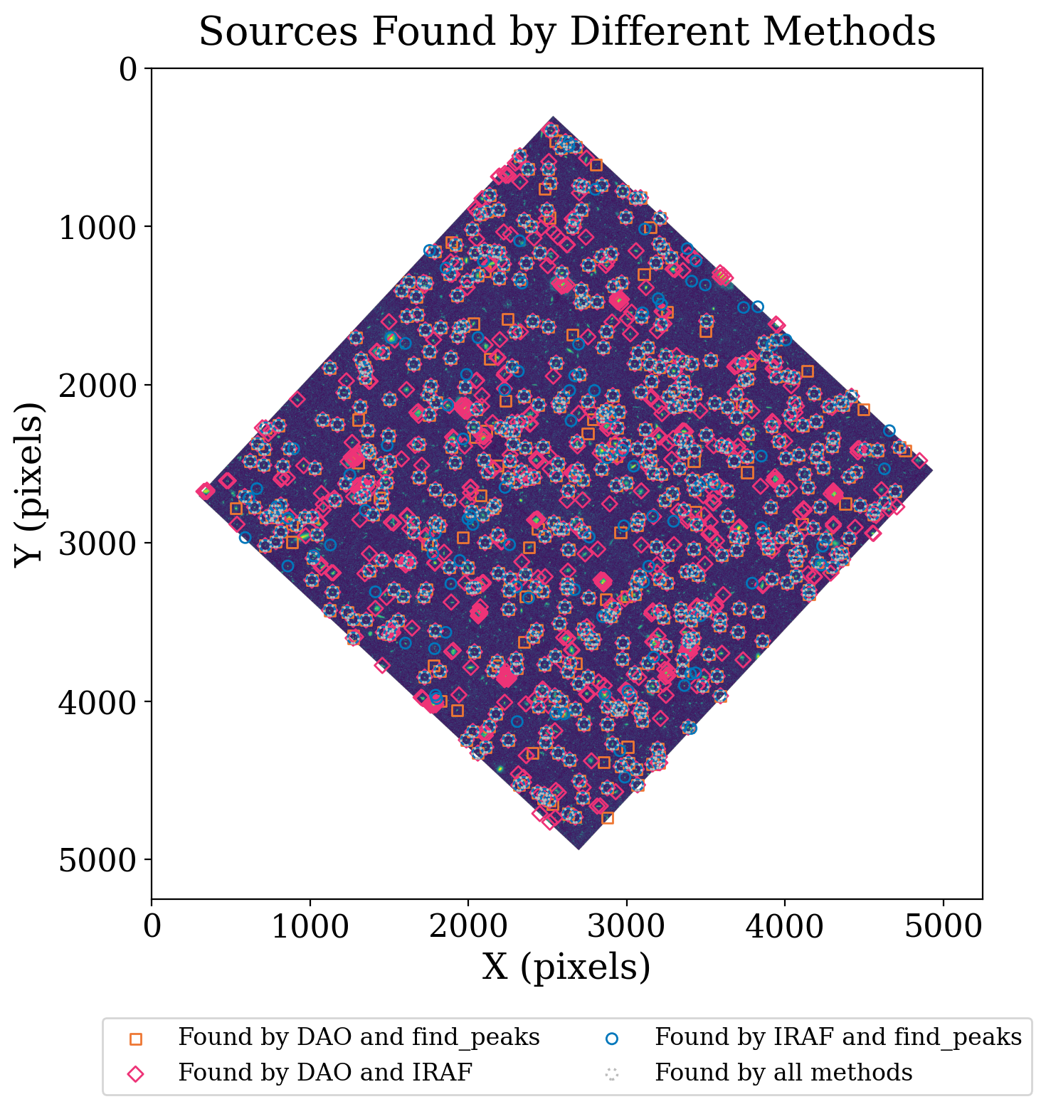
This is pretty cluttered, so we once again look at the region around the large galaxy in the image.

fig, ax1 = plt.subplots(1, 1, figsize=(8, 8))

# Plot the data
fitsplot = ax1.imshow(np.ma.masked_where(xdf_image.mask, xdf_image), norm=norm_image, alpha=0.9)

marker_size = 60
ax1.scatter(sources_findpeaks['x_peak'], sources_findpeaks['y_peak'], s=marker_size, marker='s',
            lw=1, alpha=1, facecolor='None', edgecolor='r', label='Found by find_peaks')
ax1.scatter(sources_dao['xcentroid'], sources_dao['ycentroid'], s=2 * marker_size, marker='D',
            lw=1, alpha=1, facecolor='None', edgecolor='#EE7733', label='Found by DAOfind')
ax1.scatter(sources_iraf_match['xcentroid'], sources_iraf_match['ycentroid'],
            s=4 * marker_size, marker='o', lw=1, alpha=1, facecolor='None', edgecolor='#BBBBBB',
            label="Found by IRAF starfind")

# Add legend
ax1.legend(ncol=2, loc='lower center', bbox_to_anchor=(0.5, -0.25))

top = 1125
left = 2350
cutout_size = 500

ax1.set_xlim(left, left + cutout_size)
ax1.set_ylim(top, top + cutout_size)
# Define labels
ax1.set_xlabel('X (pixels)')
ax1.set_ylabel('Y (pixels)')
ax1.set_title('Sources Found by Different Methods');

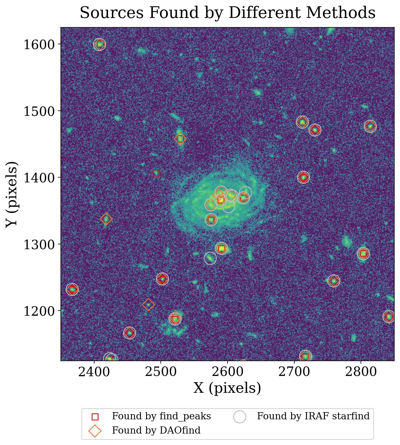
There is only one actual source in this cutout that was found by one of the star-finding techniques that were not also found by peak finding. Several sources ideintified as separate by star-finding sources in the large galaxy at the center are not actually separate. Peak finding suffers from this too but to a lesser extent.

8.3.2.4. Custom Detection Algorithms

If none of the algorithms we’ve reviewed above do exactly what you need, photutils also provides infrastructure for you to generate and use your own source detection algorithm: the StarFinderBase object can be inherited and used to develop new star-finding classes. Take a look at the documentation for more information.

If you do go that route, remember that photutils is open source; you would be very welcome to open a pull request and incorporate your new star finder into the photutils source code – for everyone to use!

8.3.2.5. Summary

The sources found by find_peaks are roughly the same as those found by the star-finding algorithms. In XX BROKEN LINK SEGMENTATION we will look at a much different approach that is especially well suited to finding extended objects.