8.2.1. IRAF-like source detection with simulated images

8.2.1.1. Overview

IRAF provided a couple of ways, starfind and daofind, to detect stellar sources in an image. photutils provides similar functionality via the DAOStarFinder and IRAFStarFinder objects

This notebook will focus on DAOStarFinder to emphasize that these options work well for detecting stars or other objects with a stellar profile. They do not work well for more extended objects.

The next couple of notebooks will:

• apply these techniques to the Hubble Extreme Deep Field, to illustrate the differences between DAOStarFinder and IRAFStarFinder, and to introduce another method of source detection,

• apply the techniques to an image of stars from a ground-based telescope, and

• illustrate other source detection techniques that work well for extended sources

8.2.1.2. Simulated image of galaxies and stars

In the first part of this notebook we consider an image that includes 100 sources, all with Gaussian profiles, some of which are fairly elongated. We used this image in the previous section about removing the background prior to source detection.

As usual, we begin with some imports.

from astropy.stats import sigma_clipped_stats, gaussian_sigma_to_fwhm
from astropy.table import QTable
from astropy.visualization import simple_norm, SqrtStretch
from astropy.visualization.mpl_normalize import ImageNormalize

import matplotlib.pyplot as plt
import numpy as np

from photutils.aperture import CircularAperture, EllipticalAperture
from photutils.datasets import make_100gaussians_image, make_gaussian_sources_image
from photutils.detection import find_peaks, DAOStarFinder

plt.style.use('../photutils_notebook_style.mplstyle')

To begin, let’s create and look the the image. We create an image normalization here that we will use for displaying the image throughout the notebook.

data = make_100gaussians_image()
norm = ImageNormalize(stretch=SqrtStretch())
plt.figure(figsize=(10, 5))
plt.imshow(data, cmap='Greys_r', origin='lower', norm=norm,
           interpolation='nearest')
plt.grid()

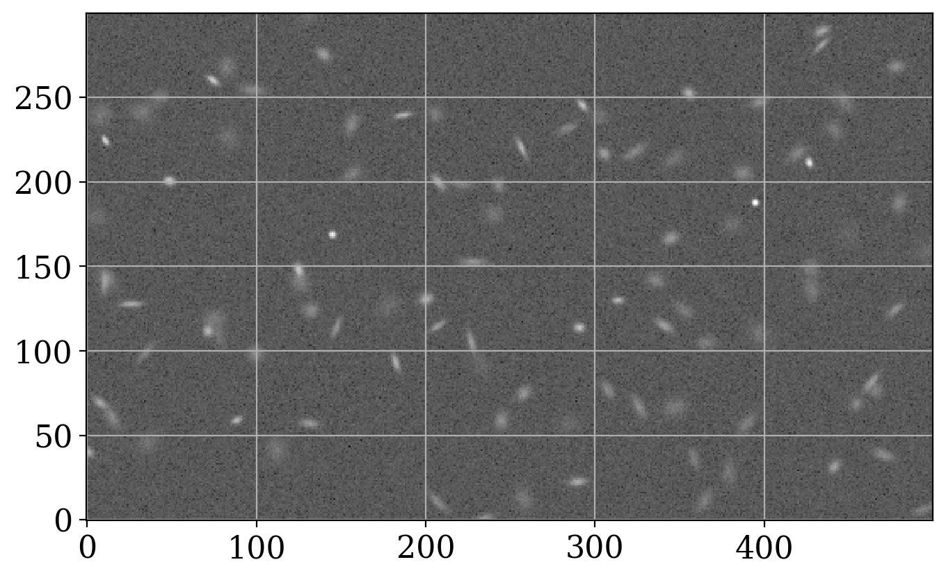
Note that some of these object are star-like – the ones that are darkest are close to circular, for example. Others are very elongated and there are a variety of brightnesses among the objects.

8.2.1.2.1. Estimate and subtract background

The background must be subtracted from the image before the sources are detected. For simplicity we estimate the sigma-clipped mean, median and standard deviation of the pixels in the image. As discussed in the section on background removal for source detection, the sigma-clipped median gives a reasonable estimate of the background in many cases.

mean, med, std = sigma_clipped_stats(data, sigma=3.0, maxiters=5)
data_subtracted = data - med

8.2.1.2.2. Detect sources

The source detection itself is a couple of lines of code:

detect_fwhm = 5.0
daofind = DAOStarFinder(fwhm=detect_fwhm, threshold=5.*std) 
sources = daofind(data_subtracted)

There are a variety of options you can select, detailed in the documentation for DAOStarFinder. We only use two for now, specifying the typical full-width half-max (FWHM) of a source, and the threshold above which to conider something a source.

A summary of the sources detected shows that DAOStarFinder detect 41 sources, substantially fewer than the 100 that are in the image.

# Format the columns to only display two decimal points 
for col in sources.colnames:  
    if col not in ('id', 'npix'):
        sources[col].info.format = '%.2f'  # for consistent table output
sources.pprint(max_width=76)  

 id xcentroid ycentroid sharpness roundness1 ... npix sky   peak flux  mag 
--- --------- --------- --------- ---------- ... ---- ---- ----- ---- -----
  1    493.85      5.95      0.57       0.61 ...   49 0.00 13.20 1.26 -0.25
  2    364.90     11.11      0.56       0.85 ...   49 0.00 12.64 1.02 -0.03
  3    441.28     31.09      0.30       0.71 ...   49 0.00 20.52 2.79 -1.11
  4    358.95     35.16      0.21      -0.00 ...   49 0.00  7.83 1.14 -0.14
  5    471.35     37.74      0.28      -0.87 ...   49 0.00 13.28 1.55 -0.48
  6    470.01     38.61      0.23      -0.90 ...   49 0.00 12.85 1.52 -0.46
  7      1.17     39.91      0.52      -0.33 ...   49 0.00 30.97 4.37 -1.60
  8    388.51     55.53      0.39       0.93 ...   49 0.00 10.42 1.01 -0.01
  9     88.64     58.82      0.47       0.55 ...   49 0.00 31.92 4.80 -1.70
 10    244.71     58.39      0.41       0.18 ...   49 0.00 17.48 1.81 -0.64
...       ...       ...       ...        ... ...  ...  ...   ...  ...   ...
 39     10.89    224.11      0.60      -0.63 ...   49 0.00 54.39 7.74 -2.22
 40    155.95    233.29      0.52       0.54 ...   49 0.00 14.74 1.19 -0.19
 41    292.63    244.96      0.54      -0.97 ...   49 0.00 38.70 5.13 -1.78
 42    397.32    246.87      0.41       0.25 ...   49 0.00 18.12 1.94 -0.72
 43    446.77    247.83      0.50      -0.22 ...   49 0.00 12.19 1.05 -0.05
 44    355.57    252.12      0.44      -0.58 ...   49 0.00 30.01 3.59 -1.39
 45     98.08    253.92      0.23       0.02 ...   49 0.00 11.16 1.31 -0.30
 46    477.97    267.93      0.36       0.12 ...   49 0.00 14.82 1.55 -0.47
 47    139.81    275.06      0.37      -0.60 ...   49 0.00 21.49 2.25 -0.88
 48    434.09    288.98      0.50       0.80 ...   49 0.00 26.73 2.85 -1.14
Length = 48 rows

A plot showing the location of all of the detected sources helps illustrate why some of sources were missed. To display where sources were detected, we create a a set of photutils circular apertures and use its plot method to add a circle over each detected source.

# CircularAperture expects a particular format for input positions...
positions = np.transpose((sources['xcentroid'], sources['ycentroid']))
apertures = CircularAperture(positions, r=detect_fwhm / 2)

plt.figure(figsize=(20, 10))
plt.imshow(data, cmap='Greys', origin='lower', norm=norm,
           interpolation='nearest')
apertures.plot(color='blue', lw=1, alpha=0.5);
plt.title("Sources detected by DAOStarFinder")

Text(0.5, 1.0, 'Sources detected by DAOStarFinder')

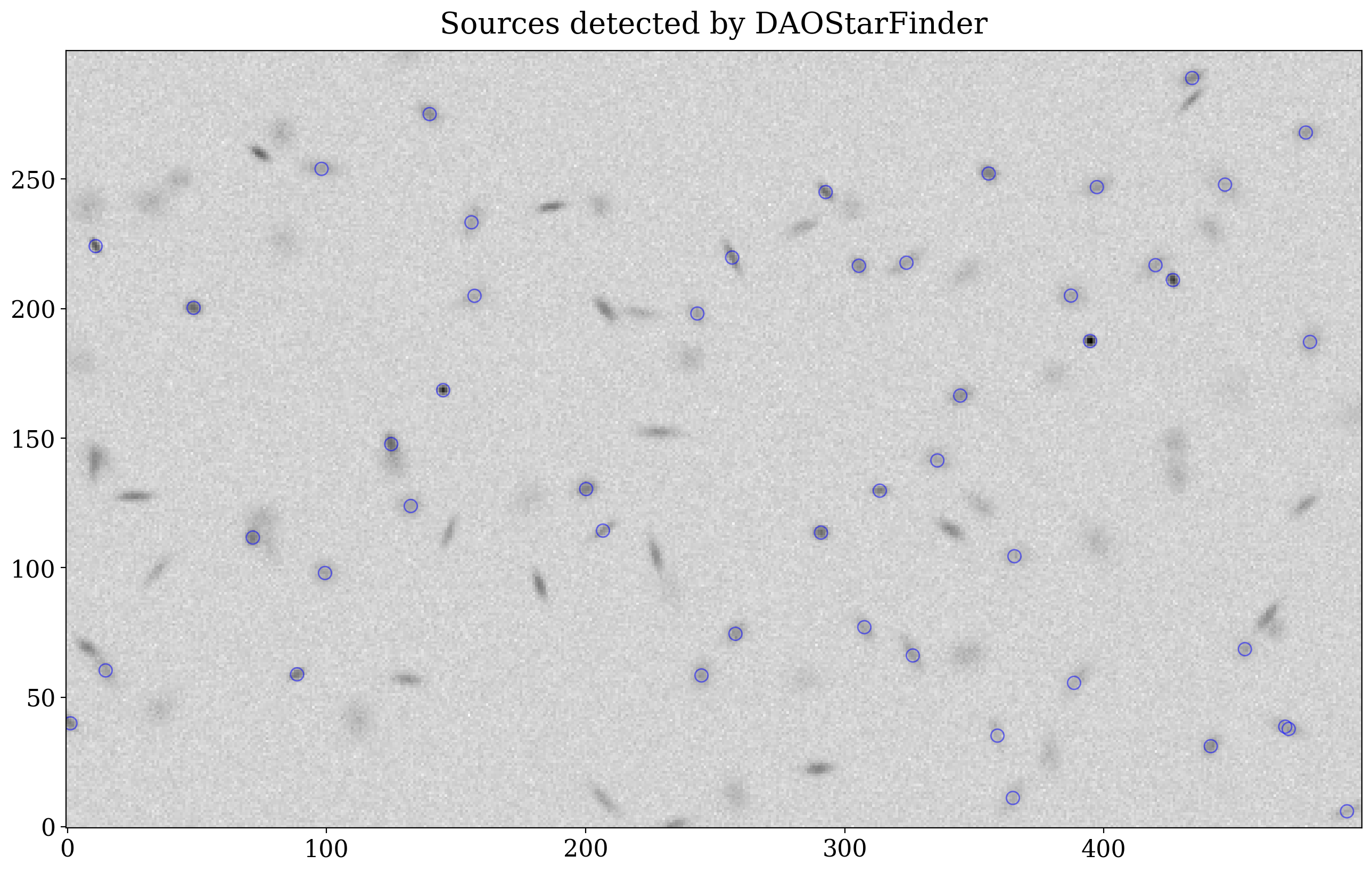
It looks like the sources that were detected are those that were not too faint and not too elongaetd.

Let’s look at the properties of the sources in this image, and explore some of the settings in DAOStarFinder to see how you could tune its parameters to detect a different subset of the sources.

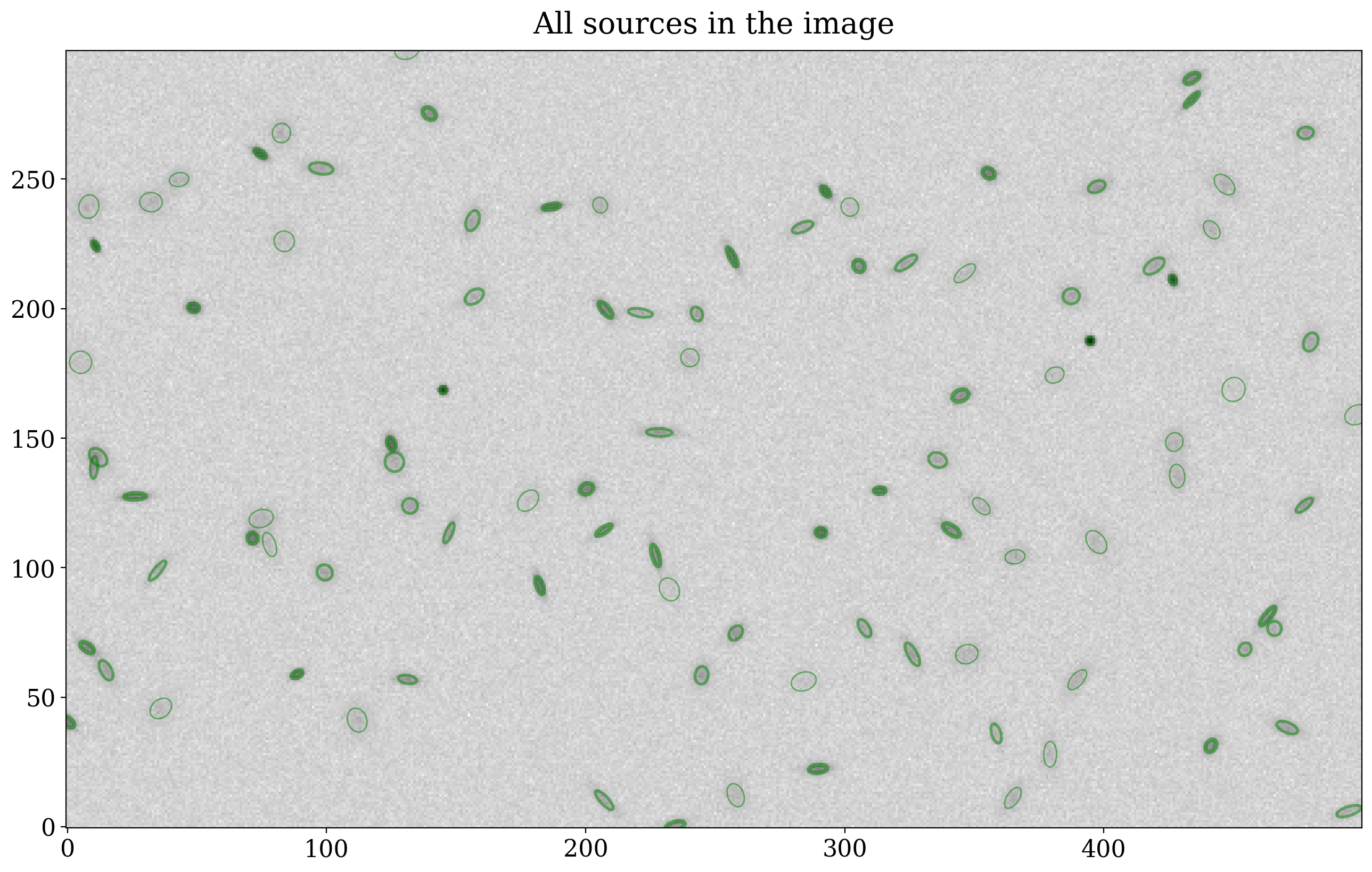
8.2.1.2.3. Sources in the image

The sources in this image are generated using the code below, which was copied from the photutils source code here.

The sources have a range of orientations, ellipticities, and widths. All of the sources are 2D Gaussians, with a FWHM ranging from roughly 3 to 15 pixels in each direction. The ratio of minor to major axis of the sources varies from 0.2 to 1.0.

n_sources = 100
flux_range = [500, 1000]
xmean_range = [0, 500]
ymean_range = [0, 300]
xstddev_range = [1, 5]
ystddev_range = [1, 5]
params = {'flux': flux_range,
          'x_mean': xmean_range,
          'y_mean': ymean_range,
          'x_stddev': xstddev_range,
          'y_stddev': ystddev_range,
          'theta': [0, 2 * np.pi]}

rng = np.random.RandomState(12345)
inp_sources = QTable()
for param_name, (lower, upper) in params.items():
    # Generate a column for every item in param_ranges, even if it
    # is not in the model (e.g., flux).  However, such columns will
    # be ignored when rendering the image.
    inp_sources[param_name] = rng.uniform(lower, upper, n_sources)
xstd = inp_sources['x_stddev']
ystd = inp_sources['y_stddev']
inp_sources['amplitude'] = inp_sources['flux'] / (2.0 * np.pi * xstd * ystd)

Let’s look at the image again, with a marker around each input source. There is quite a bit of information packed into those markers:

• the shape of the marker matches the minor-to-major axis ratio

• the major axis of the marker is the FWHM of the major axis

• the thickness of the marker edge indicates the amplitude of the source.

Next, we overlay the sources that were detected.

plt.figure(figsize=(20, 10))

# plot the image
plt.imshow(data, cmap='Greys', origin='lower', norm=norm,
           interpolation='nearest')

def plot_input_sources(ax=None, label_text=""):
    if ax is None:
        ax = plt.gca()
        
    amplitudes = sorted(inp_sources['amplitude'])
    labeled = False
    for source in inp_sources:
        minor = min(source['x_stddev'], source['y_stddev'])
        major = max(source['x_stddev'], source['y_stddev'])
        ratio = minor / major
    
        major_fwhm = major * gaussian_sigma_to_fwhm
    
        # ap = EllipticalAperture((source['x_mean'], source['y_mean']), major, minor, theta=source['theta'])
        ap = EllipticalAperture((source['x_mean'], source['y_mean']), source['x_stddev'], source['y_stddev'], theta=source['theta'])
        
        # This should give linewidths of 1, 2, or 3 given the input fluxes
        line_width = source['flux'] // 250 - 1
    
        if source['amplitude'] > amplitudes[2 * len(amplitudes) // 3]:
            line_width = 3
        elif source['amplitude'] < amplitudes[len(amplitudes) // 3]:
            line_width = 1
        else:
            line_width = 2
        # Add a label to only the first aperture plotted, otherwise each aperture will be listed individually 
        # in the legend.
        label_kw = {"label": label_text} if not labeled else {}
        labeled = True
        ap.plot(color='green', lw=line_width, alpha=0.5, ax=ax, **label_kw)

plot_input_sources()
plt.title("All sources in the image");

plt.figure(figsize=(20, 10))
# plot the image
plt.imshow(data, cmap='Greys', origin='lower', norm=norm,
           interpolation='nearest')
apertures.plot(color='blue', lw=1, alpha=1);
for idx, ap in enumerate(apertures):
    label_offset = 3
    plt.annotate(str(idx), (ap.positions[0] + label_offset, ap.positions[1] + label_offset))
plot_input_sources()
plt.title("All sources (green) and detected sources (blue)\nlabeled by detected source number");

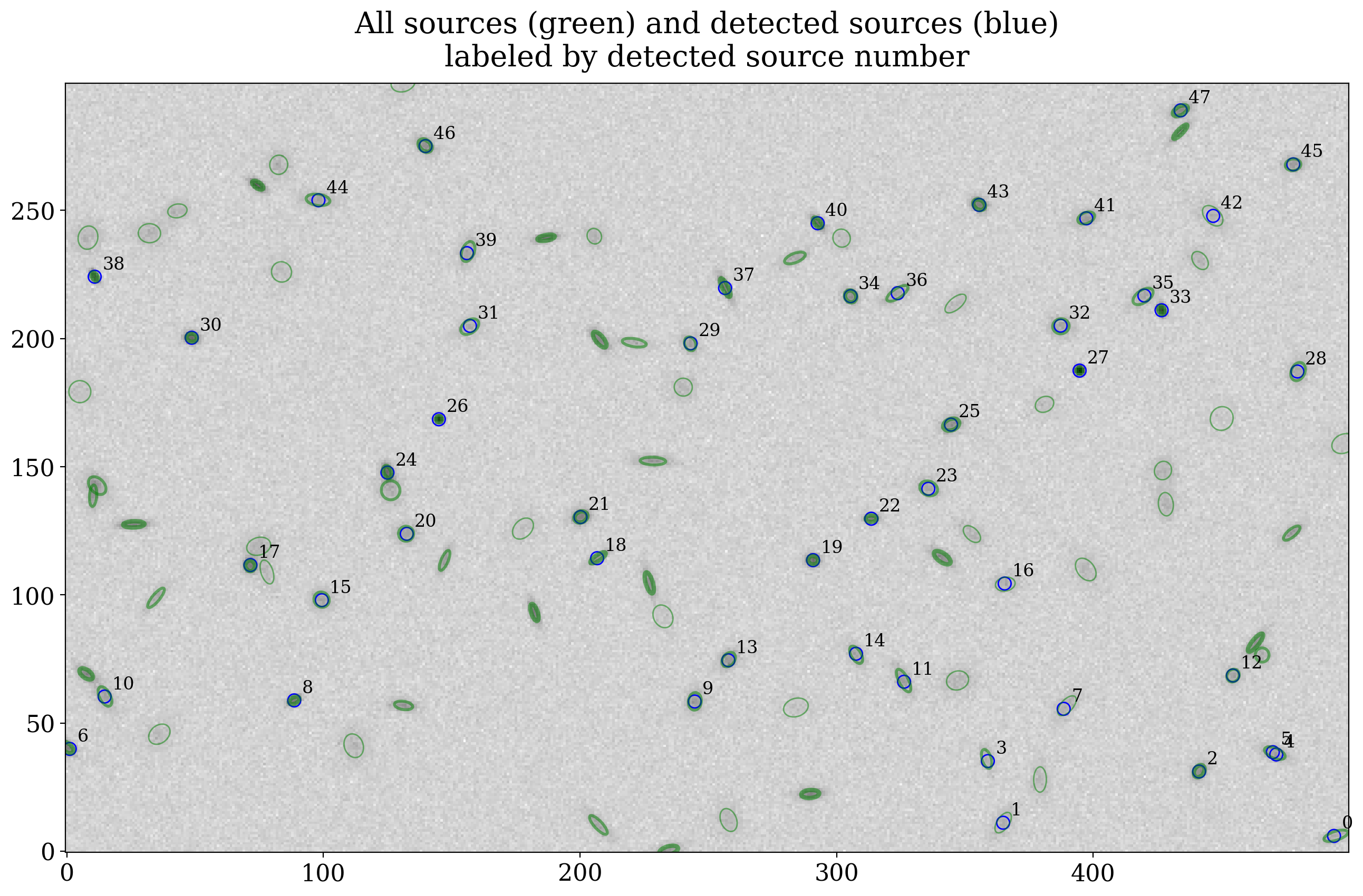
From this plot it seems that the sources detected are those that are:

• about the same size as the FWHM we input to the source finder (5 pixels in this case) – see sources labeled 5 and 22, for example.

• reasonably round or reasonably concentrated – see source 33 for an example. That source is very elongated but also very compact.

In some cases DAOStarFinder finds two sources where there is really one. Sources 5 and 6 are a good example of this.

8.2.1.2.4. An exploration of some parameters of DAOStarFinder

We can test some of the assertions in the previous paragraph. A couple of examples of that are to try

1. A lower threshold in detection to try to detect the fainter sources in this test image. Below we will try a threshold of 3 times the standard deviation of the background instead of 5 times.

2. A ratio smaller than 1 to detect the more elongated sources. The ratio argument is the ratio of the semiminor to semimajor axis. Below we will try a ratio of 0.33.

The code below begins with a function to do the plotting for this so that we can reuse that code for each plot.

def detect_sources_and_plot_apertures(data, fwhm=0, threshold_factor=5, ratio=1, ax=None, color='blue', label_text=""):
    if ax is None:
        ax = plt.gca()
        
    daofind = DAOStarFinder(fwhm=detect_fwhm, threshold=threshold_factor * std, ratio=ratio) 
    sources = daofind(data_subtracted)
    positions = np.transpose((sources['xcentroid'], sources['ycentroid']))
    apertures = CircularAperture(positions, r=detect_fwhm / 2)

    # Plot the first aperture with a label
    apertures[0].plot(color=color, lw=1, alpha=0.5, ax=ax, label=label_text)
    # Plot the rest without a label, otherwise each aperture gets its own label.
    apertures[1:].plot(color=color, lw=1, alpha=0.5, ax=ax)

fig, axes = plt.subplot_mosaic([['case 1', 'case 2']], figsize=[20, 10], sharey=True, tight_layout=True)

for ax in axes.values():
    ax.imshow(data, cmap='Greys', origin='lower', norm=norm, interpolation='nearest')
    plot_input_sources(ax=ax, label_text="input source")

# The lower threshold case
thresh = 3
detect_sources_and_plot_apertures(data_subtracted, fwhm=detect_fwhm, threshold_factor=5, ratio=1, ax=axes['case 1'], color='blue', label_text="original parameters")
detect_sources_and_plot_apertures(data_subtracted, fwhm=detect_fwhm, threshold_factor=thresh, ratio=1, ax=axes['case 1'], color='red', label_text="lower threshold")
axes['case 1'].legend(loc="upper left")
axes['case 1'].set_title(f"Source detection with threshold {thresh:.1f}")


# The small ratio case
ratio = 0.3
detect_sources_and_plot_apertures(data_subtracted, fwhm=detect_fwhm, threshold_factor=5, ratio=1, ax=axes['case 2'], color='blue', label_text="original parameters")
detect_sources_and_plot_apertures(data_subtracted, fwhm=detect_fwhm, ratio=ratio, ax=axes['case 2'], color="red", label_text="small ratio")
axes['case 2'].legend(loc="upper left")
axes['case 2'].set_title(f"Source detection with ratio {ratio:.2f}");

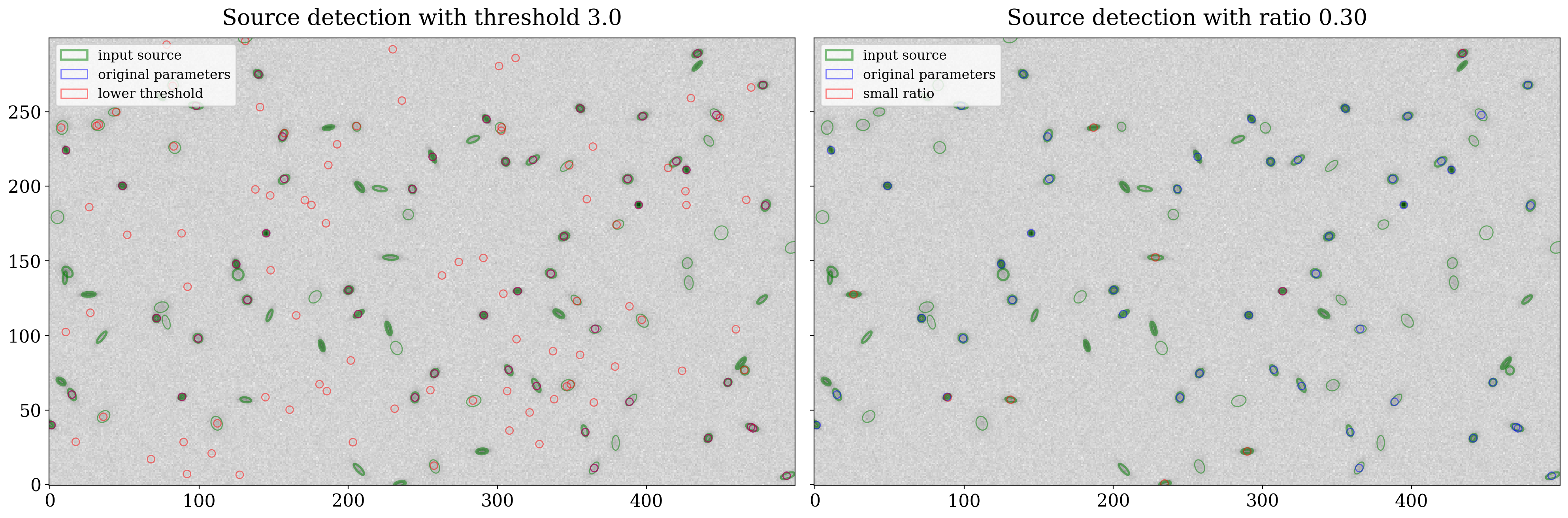
The plot on the left shows that lowering the detetion threshold does find more sources, but it also includes erroneous detections. The plot on right demonstrates that we can detect some (but not all) of the highly elongated objects by changing the ratio parameter in DAOStarFinder. The reason that we don’t pick up more of the elongated sources is that the orientation of the source matters too. The default value for the orientation is zero, i.e. aligned with the horizontal axis.

8.2.1.3. Summary

The takeway from this section should be that the IRAF-like methods implemented in photutils are good at finding star-like sources. As we will see in the next couple of sections, the methods work very well for detecting stars or galaxies that are small enough to look like stars. After that we will look at a couple of methods, local peak detection and image segmentation, that are better for detecting extended sources.