8.2.2. Detecting sources in the XDF#
8.2.2.1. Data for this notebook#
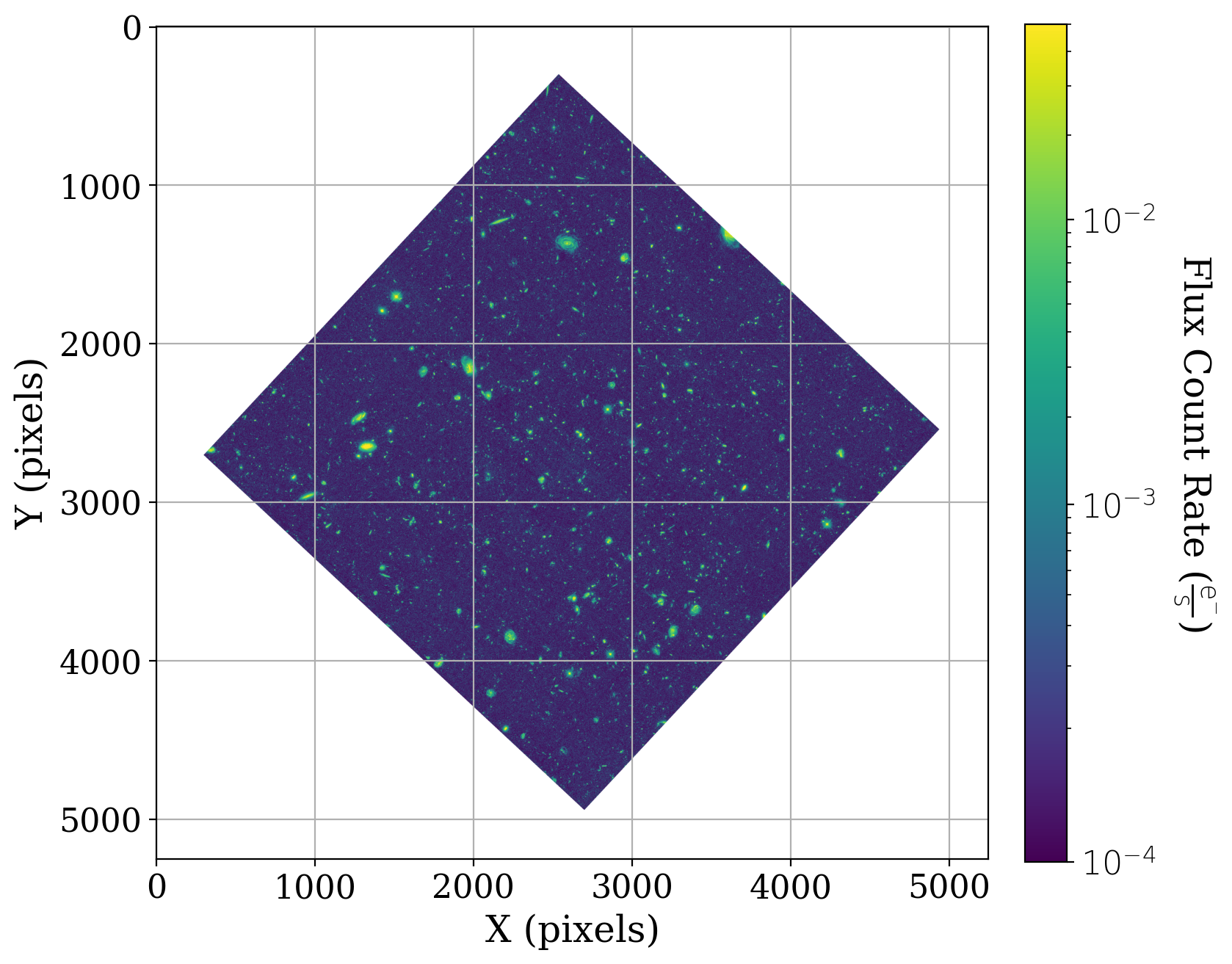
We will again be manipulating Hubble eXtreme Deep Field (XDF) data, which was collected using the Advanced Camera for Surveys (ACS) on Hubble between 2002 and 2012. The image we use here is the result of 1.8 million seconds (500 hours!) of exposure time, and includes some of the faintest and most distant galaxies that had ever been observed.
The methods demonstrated here are also available in narrative from within the photutils.detection documentation.
The original authors of this notebook were Lauren Chambers, Erik Tollerud and Tom Wilson.
8.2.2.2. Import necessary packages#
First, let’s import packages that we will use to perform arithmetic functions and visualize data:
from astropy.nddata import CCDData
from astropy.visualization import ImageNormalize, LogStretch
import matplotlib.pyplot as plt
from matplotlib.ticker import LogLocator
import numpy as np

from photutils.detection import DAOStarFinder, IRAFStarFinder

# Show plots in the notebook
%matplotlib inline
/usr/share/miniconda/envs/test/lib/python3.11/site-packages/tqdm/auto.py:21: TqdmWarning: IProgress not found. Please update jupyter and ipywidgets. See https://ipywidgets.readthedocs.io/en/stable/user_install.html
  from .autonotebook import tqdm as notebook_tqdm
Let’s also define some matplotlib parameters, such as title font size and the dpi, to make sure our plots look nice. To make it quick, we’ll do this by loading a style file shared with the other photutils tutorials into pyplot. We will use this style file for all the notebook tutorials. (See here to learn more about customizing matplotlib.)
plt.style.use('../photutils_notebook_style.mplstyle')
8.2.2.3. Data representation#
Throughout this notebook, we are going to store our images in Python using a CCDData object (see Astropy documentation), which contains a numpy array in addition to metadata such as uncertainty, masks, or units. In this case, each image has units electrons (counts) per second.
Note that you could create the CCDData object directly from the URL where this image is taken from:
url = 'https://archive.stsci.edu/pub/hlsp/xdf hlsp_xdf_hst_acswfc-60mas_hudf_f435w_v1_sci.fits'
xdf_image = CCDData.read(url)
Since the data for the guide is meant to be downloaded in bulk before going through the guide, we read the image from disk here.
xdf_image = CCDData.read('hlsp_xdf_hst_acswfc-60mas_hudf_f435w_v1_sci.fits')
As explained in a previous notebook on background estimation, it is important to mask these data, as a large portion of the values are equal to zero. We will mask out the non-data portions of the image array, so all of those pixels that have a value of zero don’t interfere with our statistics and analyses of the data.
# Define the mask
mask = xdf_image.data == 0
xdf_image.mask = mask
Let’s look at the data:
# Set up the figure with subplots
fig, ax1 = plt.subplots(1, 1, figsize=(8, 8))

# Set up the normalization and colormap
norm_image = ImageNormalize(vmin=1e-4, vmax=5e-2, stretch=LogStretch(), clip=False)
cmap = plt.get_cmap('viridis')
cmap.set_bad('white') # Show masked data as white

# Plot the data
fitsplot = ax1.imshow(np.ma.masked_where(xdf_image.mask, xdf_image),
                      norm=norm_image, cmap=cmap)

# Define the colorbar
cbar = plt.colorbar(fitsplot, fraction=0.046, pad=0.04, ticks=LogLocator())

def format_colorbar(bar):
    # Add minor tickmarks
    bar.ax.yaxis.set_minor_locator(LogLocator(subs=range(1, 10)))

    # Force the labels to be displayed as powers of ten and only at exact powers of ten
    bar.ax.set_yticks([1e-4, 1e-3, 1e-2])
    labels = [f'$10^{{{pow:.0f}}}$' for pow in np.log10(bar.ax.get_yticks())]
    bar.ax.set_yticklabels(labels)

format_colorbar(cbar)

# Define labels
cbar.set_label(r'Flux Count Rate ({})'.format(xdf_image.unit.to_string('latex')),
               rotation=270, labelpad=30)
ax1.grid()
ax1.set_xlabel('X (pixels)')
ax1.set_ylabel('Y (pixels)');
Tip: Double-click on any inline plot to zoom in.
With the DAOStarFinder class, photutils provides users with an easy application of the popular DAOFIND algorithm (Stetson 1987, PASP 99, 191), originally developed at the Dominion Astrophysical Observatory.
This algorithm detects sources by:
Searching for local maxima
Selecting only sources with peak amplitude above a defined threshold
Selecting sources with sizes and shapes that match a 2-D Gaussian kernel (circular or elliptical)
It returns:
Location of the source centroid
Parameters reflecting the source’s sharpness and roundness
Generally, the threshold that source detection algorithms use is defined as a multiple of the standard deviation. So first, we need to calculate statistics for the data:
mean, median, std = sigma_clipped_stats(xdf_image.data, sigma=3.0, maxiters=5, mask=xdf_image.mask)
---------------------------------------------------------------------------
NameError                                 Traceback (most recent call last)
Cell In[6], line 1
----> 1 mean, median, std = sigma_clipped_stats(xdf_image.data, sigma=3.0, maxiters=5, mask=xdf_image.mask)

NameError: name 'sigma_clipped_stats' is not defined
Now, let’s run the DAOStarFinder algorithm on our data and see what it finds.
daofind = DAOStarFinder(fwhm=5.0, threshold=20. * std)
sources_dao = daofind(np.ma.masked_where(xdf_image.mask, xdf_image))
print(sources_dao)
There are almost 1,500 sources detected in the image.
# Set up the figure with subplots
fig, ax1 = plt.subplots(1, 1, figsize=(8, 8))

# Plot the data
fitsplot = ax1.imshow(np.ma.masked_where(xdf_image.mask, xdf_image),
                      norm=norm_image, cmap=cmap)
ax1.scatter(sources_dao['xcentroid'], sources_dao['ycentroid'], s=30, marker='o',
            lw=1, alpha=0.7, facecolor='None', edgecolor='r')

# Define the colorbar
cbar = plt.colorbar(fitsplot, fraction=0.046, pad=0.04, ticks=LogLocator())

# format the colorbar
format_colorbar(cbar)

# Define labels
cbar.set_label(r'Flux Count Rate ({})'.format(xdf_image.unit.to_string('latex')),
               rotation=270, labelpad=30)
ax1.set_xlabel('X (pixels)')
ax1.set_ylabel('Y (pixels)')
ax1.set_title('DAOFind Sources');
Looking at a cutout around the relatively large galaxy in the top center of the image is instructive. As you can see below, the large galaxy is identified by DAOStarFinder as several overlapping sources. Some of the smaller galaxies in the image are identified as sources, but many are not. The parameters could be tuned to detect more of the sources, but it turns out there are source detection methods better suited to extended sources that will be discussed in XX BROKEN LINK XX.
fig, ax = plt.subplots(figsize=(8, 8))
top = 1125
left = 2350
cutout_size = 500
inset_display_size = 5 * cutout_size

fitsplot = ax.imshow(xdf_image, cmap=cmap, norm=norm_image, alpha=0.4)
ax.scatter(sources_dao['xcentroid'], sources_dao['ycentroid'], s=30, marker='o',
           lw=1, alpha=0.1, facecolor='None', edgecolor='r')

ax.set_xlabel('X (pixels)')
ax.set_ylabel('Y (pixels)')
ax.set_title('DAOFind Sources')

ax2 = ax.inset_axes([2600 - inset_display_size // 2, 2300, inset_display_size, inset_display_size],
                    xlim=(left, left + cutout_size), ylim=(top, top + cutout_size),
                    transform=ax.transData)
ax.indicate_inset_zoom(ax2, edgecolor="black")

ax2.imshow(xdf_image, cmap=cmap, norm=norm_image)

in_region = (
    (left < sources_dao['xcentroid']) &
    (sources_dao['xcentroid'] < (left + cutout_size)) &
    (top < sources_dao['ycentroid']) &
    (sources_dao['ycentroid'] < (top + cutout_size))
)
sources_dao_to_plot = sources_dao[in_region]
ax2.scatter(sources_dao_to_plot['xcentroid'], sources_dao_to_plot['ycentroid'], s=30, marker='o',
            lw=1, alpha=0.7, facecolor='None', edgecolor='r');
8.2.2.4. Source Detection with IRAFStarFinder#
Similarly to DAOStarFinder, IRAFStarFinder is a class that implements a pre-existing algorithm that is widely used within the astronomical community. This class uses the starfind algorithm that was originally part of IRAF.
IRAFStarFinder is fundamentally similar to DAOStarFinder in that it detects sources by finding local maxima above a certain threshold that match a Gaussian kernel. However, IRAFStarFinder differs in the following ways:
Does not allow users to specify an elliptical Gaussian kernel
Uses image moments to calculate the centroids, roundness, and sharpness of objects
Let’s run the IRAFStarFinder algorithm on our data, with the same FWHM and threshold, and see how its results differ from DAOStarFinder:
iraffind = IRAFStarFinder(fwhm=5.0, threshold=20. * std)
sources_iraf = iraffind(np.ma.masked_where(xdf_image.mask, xdf_image))
print(sources_iraf)
There are many fewer sources detected this time – only 211 compared to the almost 1500 detected by DAOStarFinder.
# Set up the figure with subplots
fig, ax1 = plt.subplots(1, 1, figsize=(8, 8))

# Plot the data
fitsplot = ax1.imshow(np.ma.masked_where(xdf_image.mask, xdf_image),
                      norm=norm_image, cmap=cmap)
ax1.scatter(sources_iraf['xcentroid'], sources_iraf['ycentroid'], s=30, marker='o',
            lw=1, alpha=0.7, facecolor='None', edgecolor='r')

# Define the colorbar
cbar = plt.colorbar(fitsplot, fraction=0.046, pad=0.04, ticks=LogLocator())

# format the colorbar
format_colorbar(cbar)

# Define labels
cbar.set_label(r'Flux Count Rate ({})'.format(xdf_image.unit.to_string('latex')),
               rotation=270, labelpad=30)
ax1.set_xlabel('X (pixels)')
ax1.set_ylabel('Y (pixels)')
ax1.set_title('IRAFFind Sources');
Looking at a cutout around the relatively large galaxy in the top center of the image is again instructive and gives a hint as to some of the differences between DAOStarFinder and IRAFStarFinder.
There are several differences. The large galaxy is now identified as a single source, but many fewer sources are detected overall. The sources aside from the large galaxy that are detected are ones that are point-like.
fig, ax = plt.subplots(figsize=(8, 8))
top = 1125
left = 2350
cutout_size = 500
inset_display_size = 5 * cutout_size

fitsplot = ax.imshow(xdf_image, cmap=cmap, norm=norm_image, alpha=0.4)
ax.scatter(sources_iraf['xcentroid'], sources_iraf['ycentroid'], s=30, marker='o',
           lw=1, alpha=0.1, facecolor='None', edgecolor='r')

ax.set_xlabel('X (pixels)')
ax.set_ylabel('Y (pixels)')
ax.set_title('IRAF Starfind Sources')

ax2 = ax.inset_axes([2600 - inset_display_size // 2, 2300, inset_display_size, inset_display_size],
                    xlim=(left, left + cutout_size), ylim=(top, top + cutout_size),
                    transform=ax.transData)
ax.indicate_inset_zoom(ax2, edgecolor="black")

ax2.imshow(xdf_image, cmap=cmap, norm=norm_image)

in_region = (
    (left < sources_iraf['xcentroid']) &
    (sources_iraf['xcentroid'] < (left + cutout_size)) &
    (top < sources_iraf['ycentroid']) &
    (sources_iraf['ycentroid'] < (top + cutout_size))
)
sources_iraf_to_plot = sources_iraf[in_region]
ax2.scatter(sources_iraf_to_plot['xcentroid'], sources_iraf_to_plot['ycentroid'], s=30, marker='o',
            lw=1, alpha=0.7, facecolor='None', edgecolor='r');
8.2.2.5. Comparing DAOStarFinder and IRAFStarFinder#
You might have noticed that the IRAFStarFinder algorithm only found 211 sources in our data – 14% of what DAOStarFinder found. Why is this?
The answer comes down to the default settings for the two algorithms: (1) there are differences in the upper and lower bounds on the requirements for source roundness and sharpness, and (2) IRAFStarFinder includes a minimum separation between sources that DAOStarFinder does not have:
|
|
|
|---|---|---|
sharplo |
0.5 |
0.2 |
sharphi |
2.0 |
1.0 |
roundlo |
0.0 |
-1.0 |
roundhi |
0.2 |
1.0 |
minsep_fwhm |
1.5 * FWHM |
N/A |
Thinking about this, it then makes sense that IRAFStarFinder would find fewer sources. It has tighter restrictions on source roundness and sharplo, meaning that it eliminates more elliptical galactic sources (this is the eXtreme Deep Field, after all!), and the minimum separation requirement further rules out sources that are too close to one another.
If we set all these parameters to be equivalent, though, we should find much better agreement between the two methods:
iraffind_match = IRAFStarFinder(fwhm=5.0, threshold=20. * std,
                                sharplo=0.2, sharphi=1.0,
                                roundlo=-1.0, roundhi=1.0,
                                minsep_fwhm=0.0)
sources_iraf_match = iraffind_match(np.ma.masked_where(xdf_image.mask, xdf_image))
print(sources_iraf_match)
The number of detected sources are in much better agreement now – 1415 versus 1470 – but the improved agreement can also be seen by plotting the location of these sources:
# Set up the figure with subplots
fig, [ax1, ax2] = plt.subplots(1, 2, figsize=(12, 6))
plt.tight_layout()

# Plot the DAOStarFinder data
fitsplot = ax1.imshow(np.ma.masked_where(xdf_image.mask, xdf_image),
                      norm=norm_image, cmap=cmap)
ax1.scatter(sources_dao['xcentroid'], sources_dao['ycentroid'], s=30, marker='o',
            lw=1, alpha=0.7, facecolor='None', edgecolor='r')
ax1.set_xlabel('X (pixels)')
ax1.set_ylabel('Y (pixels)')
ax1.set_title('DAOStarFinder Sources')

# Plot the IRAFStarFinder data
fitsplot = ax2.imshow(np.ma.masked_where(xdf_image.mask, xdf_image),
                      norm=norm_image, cmap=cmap)
ax2.scatter(sources_iraf_match['xcentroid'], sources_iraf_match['ycentroid'],
            s=30, marker='o', lw=1, alpha=0.7, facecolor='None', edgecolor='r')
ax2.set_xlabel('X (pixels)')
ax2.set_title('IRAFStarFinder Sources')

# Define the colorbar
cbar_ax = fig.add_axes([1, 0.09, 0.03, 0.87])
cbar = plt.colorbar(fitsplot, cbar_ax, fraction=0.046, pad=0.04, ticks=LogLocator())

# format the colorbar
format_colorbar(cbar)

cbar.set_label(r'Flux Count Rate ({})'.format(xdf_image.unit.to_string('latex')),
               rotation=270, labelpad=30);
Take this example as reminder to be mindful when selecting a source detection algorithm, and when defining algorithm parameters! Don’t be afraid to play around with the parameters and investigate how that affects your results.
The detailed view near the large galaxy confirms that the results are now nearly identical.
# Set up the figure with subplots
fig, [ax1, ax2] = plt.subplots(1, 2, figsize=(12, 6))
plt.tight_layout()

# Plot the DAOStarFinder data
fitsplot = ax1.imshow(np.ma.masked_where(xdf_image.mask, xdf_image),
                      norm=norm_image, cmap=cmap)
ax1.scatter(sources_dao['xcentroid'], sources_dao['ycentroid'], s=30, marker='o',
            lw=1, alpha=1, facecolor='None', edgecolor='r')
ax1.set_xlabel('X (pixels)')
ax1.set_ylabel('Y (pixels)')
ax1.set_title('DAOStarFinder Sources')
ax1.set_xlim(left, left + cutout_size)
ax1.set_ylim(top, top + cutout_size)

# Plot the IRAFStarFinder data
fitsplot = ax2.imshow(np.ma.masked_where(xdf_image.mask, xdf_image),
                      norm=norm_image, cmap=cmap)
ax2.scatter(sources_iraf_match['xcentroid'], sources_iraf_match['ycentroid'],
            s=30, marker='o', lw=1, alpha=1, facecolor='None', edgecolor='r')
ax2.set_xlabel('X (pixels)')
ax2.set_title('IRAFStarFinder Sources')
ax2.set_xlim(left, left + cutout_size)
ax2.set_ylim(top, top + cutout_size)

# Define the colorbar
cbar_ax = fig.add_axes([1, 0.09, 0.03, 0.87])
cbar = plt.colorbar(fitsplot, cbar_ax, fraction=0.046, pad=0.04, ticks=LogLocator())
fig.suptitle("Cutout near large galaxy", fontsize=20, y=1.1)
# format the colorbar
format_colorbar(cbar)

cbar.set_label(r'Flux Count Rate ({})'.format(xdf_image.unit.to_string('latex')),
               rotation=270, labelpad=30);
8.2.2.6. Summary#
Both DAOStarFinder and IRAFStarFinder are capable of producing similar results if the input parameters are matched. One noticable difference between them is that IRAFStarFinder includes a parameter for setting a minimum separation of sources. This is particularly useful to exclude overlapping sources if the intent is to perform aperture photometry.
In the section XX BROKEN LINK XX the detection methods discussed here will be compared with local peak detection, which performs better on extended sources. Section XX BROKEN LINK SEGMENTATIONXX will demonstrate using image segmentation to detect sources. That also performs better on extended sources than the star finders described in this notebook.