8.3.3. Peak finding in a stellar image#
8.3.3.1. Data used in this notebook#
The image in this notebook is of the field of the star TIC 125489084 on a night when the moon was nearly full. The moonlight caused a smooth gradient across the background of the image.
As discussed in the section about background subtraction with this image, the best way to remove the background in this case is to use photutils to construct a 2D model of the background.
As we will see in a moment, DAOStarFinder does a good job identifying most of the sources in the image, since all of the sources are stars.
import warnings

from astropy.nddata import CCDData
from astropy.stats import sigma_clipped_stats, SigmaClip
from astropy.visualization.mpl_normalize import AsymmetricPercentileInterval, ImageNormalize

import matplotlib.pyplot as plt
import numpy as np

from photutils.background import Background2D, MeanBackground
from photutils.centroids import centroid_2dg
from photutils.detection import find_peaks, DAOStarFinder

plt.style.use('../photutils_notebook_style.mplstyle')
/usr/share/miniconda/envs/test/lib/python3.11/site-packages/tqdm/auto.py:21: TqdmWarning: IProgress not found. Please update jupyter and ipywidgets. See https://ipywidgets.readthedocs.io/en/stable/user_install.html
  from .autonotebook import tqdm as notebook_tqdm
To begin, let’s create the image and subtract the background. Recall that this image contains only stars.
ccd_image = CCDData.read('TIC_125489084.01-S001-R055-C001-ip.fit.bz2')

sigma_clip = SigmaClip(sigma=3., maxiters=5)
bkg_estimator = MeanBackground()
bkg = Background2D(ccd_image, box_size=200, filter_size=(9, 9), mask=ccd_image.mask,
                   sigma_clip=sigma_clip, bkg_estimator=bkg_estimator)
# Calculate the 2D background subtraction, maintaining metadata, unit, and mask
ccd_2d_bkgdsub = ccd_image.subtract(bkg.background)

data_subtracted = ccd_2d_bkgdsub.data
WARNING: FITSFixedWarning: RADECSYS= 'FK5 ' / Equatorial coordinate system
the RADECSYS keyword is deprecated, use RADESYSa. [astropy.wcs.wcs]
mean, med, std = sigma_clipped_stats(data_subtracted, sigma=3.0, maxiters=5)
8.3.3.2. Source Detection with peak finding#
As in the previous two peak finding examples, we include a centroid function so that we can compare the sources detected by peak finding with the sources identified by the star-finding algorithms.
The centroid-finding, which we do here only so that we can compare positions found by this method to positions found by the star-finding methods, can generate many warnings when an attempt is made to fit a 2D Gaussian to the sources. The warnings are suppressed below to avoid cluttering the output.
with warnings.catch_warnings(action="ignore"):
    sources_findpeaks = find_peaks(data_subtracted,
                                   threshold=5. * std, box_size=29,
                                   centroid_func=centroid_2dg)
print(sources_findpeaks)
 id x_peak y_peak   peak_value        x_centroid           y_centroid
--- ------ ------ ------------- --------------------- -------------------
  1    594      9     75.484314     603.3703872401995 -49.574109694658816
  2      0     11 1.1987588e+06   -138.81731672630772   43.45733947806261
  3    351     11     246.65854    351.35681571228605  11.195530916361045
  4   2437     19     145.94908     2436.787838335382  18.997759494071353
  5    114     25      75.18233    113.54243542523396  26.724869786122554
  6    820     58     287.01605     820.2714101000864   57.61873898452343
  7   2950     83     136.11548     2944.737283463667    84.3801659191927
  8   3582     91     13919.255    3581.7095598877872   91.03616705939224
  9      0     97      407317.2     680.8898185712477   675.8954457901926
 10   1066    103     398.52728    1054.6981876617374   80.43008655935569
...    ...    ...           ...                   ...                 ...
543    674   4023     240.61124     672.8288347709151  4024.0451993829365
544      0   4029      176856.3     3550.346826110882    9130.63407583919
545    905   4038      77.64653     865.4867169098237  4020.5455655186383
546   2093   4049     170.61674    2092.3829693205507  4049.6421876307954
547   1640   4056     198.92299    1640.0074527423876   4055.604347909178
548      0   4060 1.2422764e+06 -0.011927489313353051  4060.1534315514295
549   2214   4071     78.925705    2212.4367632453677  4072.6693006756855
550    623   4073      155.9338      622.893406969961  4073.8168815566223
551      0   4079     401068.72 -0.019912592828290627  4076.5176931361716
552   3994   4080      74.31587    3992.0851518324234    4081.83552062658
Length = 552 rows
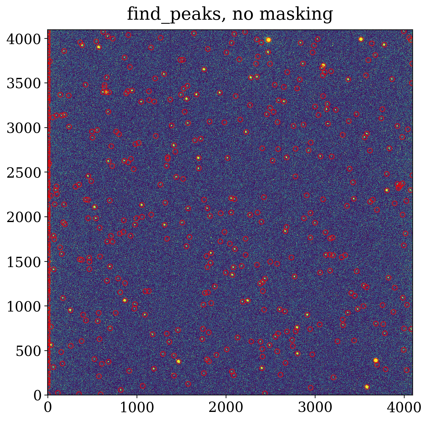
The roughly 550 sources identified by find_peaks is much larger than the number detected by the star-finding approach.
Let’s take a look at the detections on the image to see what is going on.
# Set up the figure with subplots
fig, ax1 = plt.subplots(1, 1, figsize=(8, 8))

# Plot the 2D-subtracted data
norm = ImageNormalize(ccd_2d_bkgdsub, interval=AsymmetricPercentileInterval(30, 99.5))

fitsplot = ax1.imshow(data_subtracted, cmap='viridis', origin='lower', norm=norm,
           interpolation='nearest')
ax1.scatter(sources_findpeaks['x_peak'], sources_findpeaks['y_peak'], s=30, marker='o',
            lw=1, alpha=0.7, facecolor='None', edgecolor='r')
ax1.set_title("find_peaks, no masking")
Text(0.5, 1.0, 'find_peaks, no masking')
8.3.3.2.1. Mask bad regions of the CCCD#
The column on the left side of this CCD is not actually exposed to light, so find_peaks finds a bunch of spurious sources. Recall that we can provide a mask to the source finder. As we did in the star-finding approach, we exclude the region within 50 pixels of the edge.
# Create a mask array
mask = np.zeros_like(ccd_2d_bkgdsub, dtype=bool)

# Set the mask for a border of 50 pixels around the image
mask[:50, :] = mask[-50:, :] = mask[:, :50] = mask[:, -50:] = 1.0

with warnings.catch_warnings(action="ignore"):
    sources_findpeaks = find_peaks(data_subtracted, mask=mask,
                                   threshold=5. * std, box_size=29,
                                   centroid_func=centroid_2dg)
# Set up the figure with subplots
fig, ax1 = plt.subplots(1, 1, figsize=(8, 8))

# Plot the 2D-subtracted data
norm = ImageNormalize(ccd_2d_bkgdsub, interval=AsymmetricPercentileInterval(30, 99.5))

fitsplot = ax1.imshow(data_subtracted, cmap='viridis', origin='lower', norm=norm,
           interpolation='nearest')
ax1.scatter(sources_findpeaks['x_peak'], sources_findpeaks['y_peak'], s=30, marker='o',
            lw=1, alpha=0.7, facecolor='None', edgecolor='r')

ax1.set_title("find_peaks, image edges masked");
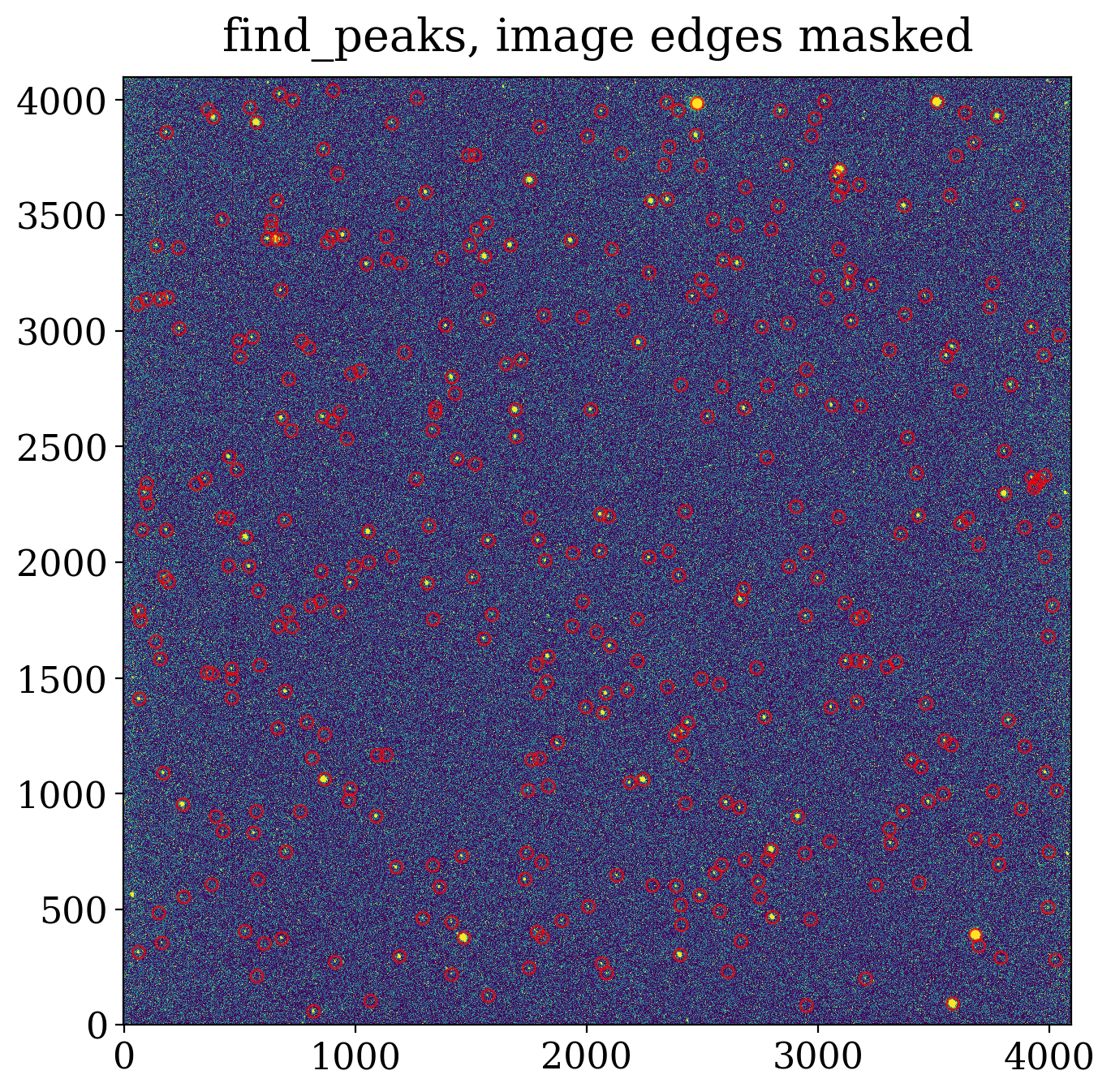
This looks quite a bit more reasonable.
8.3.3.3. Comparing Detection Methods#
Let’s compare how peak finding compares to using DAOStarFinder on this image.
# Create the star finder
fwhm = 6.2
daofinder = DAOStarFinder(threshold=5 * std, fwhm=2 * fwhm)
sources_dao = daofinder(ccd_2d_bkgdsub.data, mask=mask)
print(f'''DAOStarFinder: {len(sources_dao)} sources
find_peaks: {len(sources_findpeaks)} sources''')
DAOStarFinder: 442 sources
find_peaks: 389 sources
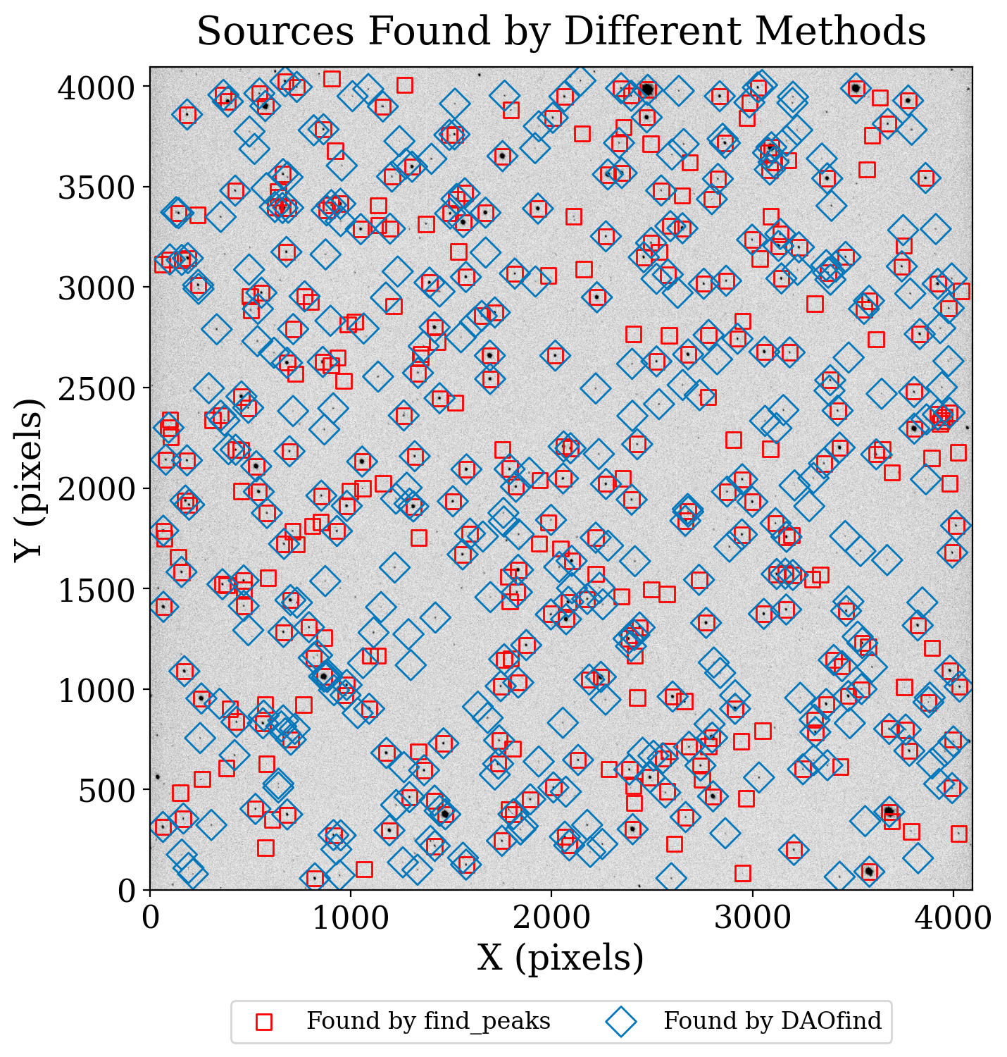
In this example, many more sources are detected by DAOStarFinder than by find_peaks. A plot showing both detection methods illustrates that the star-finding approach is doing a better job here.
fig, ax1 = plt.subplots(1, 1, figsize=(8, 8))

# Plot the data
fitsplot = ax1.imshow(data_subtracted, norm=norm, cmap='Greys', origin='lower')

marker_size = 60
ax1.scatter(sources_findpeaks['x_peak'], sources_findpeaks['y_peak'], s=marker_size, marker='s',
            lw=1, alpha=1, facecolor='None', edgecolor='r', label='Found by find_peaks')
ax1.scatter(sources_dao['xcentroid'], sources_dao['ycentroid'], s=2 * marker_size, marker='D',
            lw=1, alpha=1, facecolor='None', edgecolor='#0077BB', label='Found by DAOfind')

# Add legend
ax1.legend(ncol=2, loc='lower center', bbox_to_anchor=(0.5, -0.20))


ax1.set_xlabel('X (pixels)')
ax1.set_ylabel('Y (pixels)')
ax1.set_title('Sources Found by Different Methods');
8.3.3.4. Summary#
In this case, DAOStarFinder performs better than find_peaks. This makes sense, since DAOStarFinder is tuned for finding stars, and all of the sources in this image are stars.