About bias and overscan
Contents
2.1. About bias and overscan#
2.1.1. Sample bias images#
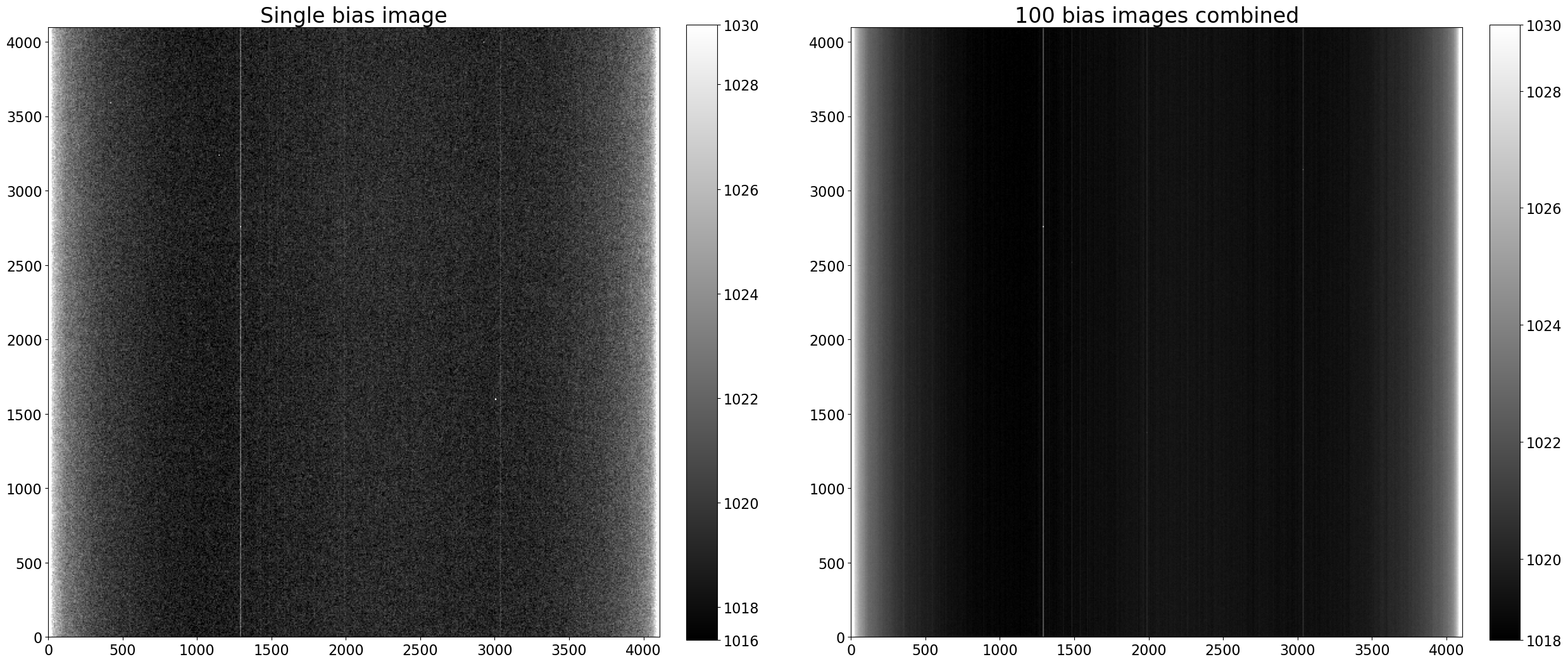
The images below are a single bias frame and an average 100 bias frames from an Andor Apogee Aspen CG16M, a low-end 4k × 4k CCD with a Kodak KAF-16803 sensor chip. That model camera has a typical bias level around 1000 and read noise around 10 \(e^-\), though the precise value varies from camera to camera and with temperature.
%load_ext autoreload
%autoreload 2
%matplotlib inline
import matplotlib.pyplot as plt
# Use custom style for larger fonts and figures
plt.style.use('guide.mplstyle')
from astropy.nddata import CCDData
from astropy.visualization import hist

import numpy as np

from convenience_functions import show_image
one_bias = CCDData.read('single_bias_thermoelectric.fit.bz2', unit='adu')
one_hundred_bias = CCDData.read('combined_bias_100_images.fit.bz2', unit='adu')
WARNING: FITSFixedWarning: 'datfix' made the change 'Set MJD-OBS to 58270.549444 from DATE-OBS'. [astropy.wcs.wcs]
INFO: using the unit adu passed to the FITS reader instead of the unit adu in the FITS file. [astropy.nddata.ccddata]
WARNING: FITSFixedWarning: 'datfix' made the change 'Set MJD-OBS to 58269.954861 from DATE-OBS'. [astropy.wcs.wcs]
fig, (ax_1_bias, ax_avg_bias) = plt.subplots(1, 2, figsize=(30, 15))

show_image(one_bias.data, cmap='gray', ax=ax_1_bias, fig=fig, input_ratio=8)
ax_1_bias.set_title('Single bias image')
show_image(one_hundred_bias.data, cmap='gray', ax=ax_avg_bias, fig=fig, input_ratio=8)
ax_avg_bias.set_title('100 bias images combined');
2.1.1.1. Note a few things#
The bias level in this specific camera is about 1023 (the mid-range of the colorbar).
The image is brighter on the left and right edges. This “amplifier glow” is frequently present and caused by the CCD electronics (photosensors with an applied voltage are LEDs).
There are several vertical lines; these are columns for which the bias level is consistently higher.
There is noticeable “static” in the images; that is read noise.
None of the variations are particularly large.
Combining several bias images vastly reduces the read noise. This example is a little unrealistic in that 100 bias images were combined, but it still illustrates the idea that combining images reduces noise.
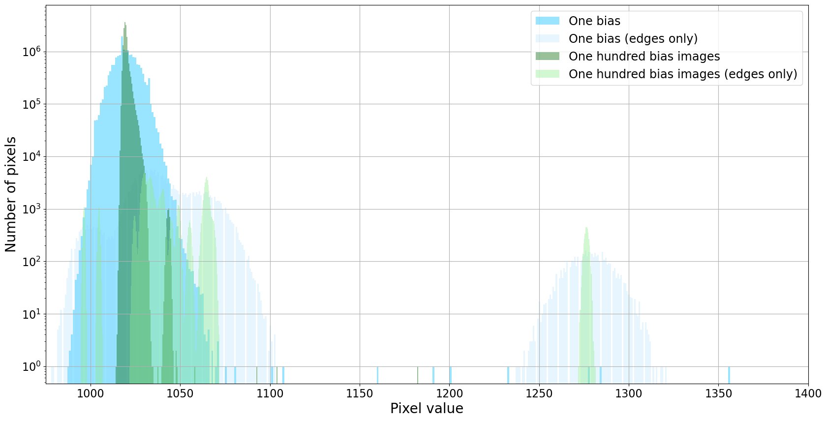
2.1.2. Impact of combining images on noise#
As discussed at length in the notebook on combination, the reason for taking and combining several calibration images is to reduce the noise if the images are used for calibration. The difference between a single image and a combination of images is apparent in the images above. Another way to see the impact of combining images is in the histogram of pixel values. Notice that the distribution of values is much narrower for the combined image than for a single bias. Pixels near the edges, where the amplifier glow is large, are binned separately from the rest of the pixels to emphasize the uniformity of the chip away from the glow.
plt.figure(figsize=(20, 10))
hist(one_bias.data[:, 15:-30].flatten(), bins=800, alpha=0.4, label='One bias', color='deepskyblue')
hist(np.concatenate((one_bias.data[:, :15].flatten(), one_bias.data[:, -30:].flatten())), bins=400, alpha=0.2, label='One bias (edges only)', color='lightskyblue')
#hist(, bins=800, alpha=0.2, label='One bias (edges only)', color='darkblue')
hist(one_hundred_bias.data[:, 15:-30].flatten(), bins=800, alpha=0.4, label='One hundred bias images', color='darkgreen')
hist(np.concatenate((one_hundred_bias.data[:, :15].flatten(), one_hundred_bias.data[:, -30:].flatten())), bins=800, alpha=0.4, label='One hundred bias images (edges only)', color='lightgreen')

#hist(one_hundred_bias.data[:, :15].flatten(), bins=800, alpha=0.4, label='One hundred bias images', color='darkgreen')

plt.grid()
plt.xlim(975, 1400)
plt.legend()
plt.xlabel('Pixel value')
plt.ylabel('Number of pixels')
plt.semilogy();
2.1.3. Bias calibration overview#
The progression here is to “calibrate” the bias images by subtracting overscan, if desired, trim the overscan from the bias images if it is present, and combine all of the bias images to make a “combined” bias (another common term for these images is “master” bias and occasionally “super” bias).